Hyperspectral data

The Hypervision SDK is built for processing hyperspectral image data. Therefore, it is important to understand some properties of this data before looking at the SDK itself, in particular, what hyperspectral images are and how they differ from regular images.

See also

This guide covers how hyperspectral images are represented as data and how manipulating them relates to and differs from regular grayscale or RGB images. For a detailed introduction to hyperspectral imaging, refer to the detailed guide on our main documentation page.

A hyperspectral image is like a regular RGB image but with many more color channels, usually hundreds. It is therefore convenient and appropriate to understand hyperspectral images as three-dimensional arrays. While RGB images are also three-dimensional, we usually don’t think of them as such because they visually appear two-dimensional and we mostly operate on them from a spatial perspective. Hyperspectral images, on the other hand, operate on both spatial and spectral dimensions, depending on what kind of information we wish to extract from them. Due to their inherent three-dimensional structure, hyperspectral images are often referred to as data cubes.

A hyperspectral image \(H\) is an \(L\times S\times B\) array, where \(L\) is the spatial height (denoted lines), \(S\) is the spatial width (denoted samples), and \(B\) is the spectral depth (denoted bands).

See also

The convention of denoting the height lines and the width samples is likely a result of the terminology being informed by the image capturing method used by most hyperspectral cameras. You can read more about the different types in our main documentation page.

Using this notation, we can recover a regular grayscale image \(I_b\) for a given spectral band \(b\) as follows:

\[\begin{split}I_{b} = \begin{bmatrix} H_{1,1,b} & \dots & H_{1,S,b}\\ \vdots & \ddots & \vdots\\ H_{L,1,b} & \dots & H_{L,S,b} \end{bmatrix}\end{split}\]

We can recover a single spectrum \(S_{l,s}\) at a specified line \(l\) and sample \(s\) with:

\[S_{l,s} = \begin{bmatrix}H_{l,s,1} & \dots & H_{l,s,B}\end{bmatrix}\]

Tip

It is useful to think of a hyperspectral image as either a stack of grayscale images or as a two-dimensional array of spectra.

Memory layout

With regular RGB images, we rarely think of the memory representation because the low number of channels results in relatively contiguous memory no matter what is operated on. This is not the case for hyperspectral images. As shown above, operating on either a spatial slice or individual spectra may require reading memory locations spaced far apart. Additionally, apart from snapshot hyperspectral cameras, the raw camera data is naturally formatted as planar slices of a full data cube. Depending on what type of camera is used, the natural memory format will be different.

In HSI, we operate with three memory orderings: BSQ (band sequential), BIL (band interleaved by line), and BIP (band interleaved by pixel). The ordering of a particular data cube is referred to as its interleave. BSQ is like a stack of grayscale images and BIP is similar to how RGB is stored in many file formats (for example PNG), with the channels of each pixel being contiguous. BIL is in between. When using the size notation for three-dimensional arrays, the format sizes can be described as:

\[\begin{split}BSQ = B\times L\times S\\ BIL = L\times B\times S\\ BIP = L\times S\times B\end{split}\]

See also

The main documentation page contains further information and examples of memory orderings.

The memory orderings can be visualised as the sides of a three-dimensional cube as shown in Fig. 1

Fig. 1 This diagram illustrates how the three interleave types dictate the in-memory layout of HSI files. The top box describes the order in which each axis is laid out in memory. Elements in “0” are consecutive.

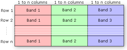
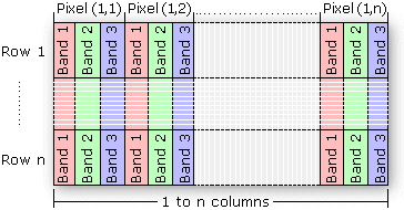
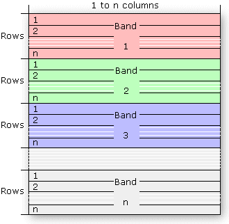
Each format can be visualised in two dimensions using color to represent the band axis as shown in Fig. 2, Fig. 3, and Fig. 4. This visualisation might give a more intuitive sense of what format is needed for a given situation.

Fig. 2 A BSQ example file. It is like a stack of grayscale images for each band.

Fig. 3 A BIP example file. This is how a regular RGB image is usually stored. The data for each pixel is consecutive.

Fig. 4 A BIL example file. Each horizontal line is consecutive in memory for a given band.

Interleave conversion

Converting between the formats is simple but can get confusing. The diagram below illustrates how one transforms from each of the formats to any other.

Fig. 5 The figure is a reference for determining how to permute axes from one format to another.