Hyperspectral Imaging
Hyperspectral Camera - Explainer from The University of Southern Denmark, SDU (in cooperation with Newtec/Qtec)
Electromagnetic spectrum
The visible light spectrum for human vision is relatively narrow, spanning only from around 380 nm (violet) to about 750 nm (red). However, the whole electromagnetic spectrum covers a much larger range, spanning beyond ultraviolet and infrared to include x-rays, gamma waves, microwave and radio waves.
RGB cameras will normally only cover the visible light spectrum. However there are more specialized cameras that can capture parts of the infrared (NIR, SWIR, ...) and/or ultraviolet spectrums as well (and even x-rays). The "invisible" parts of the spectrum can be quite useful for detecting features that are generally related to the chemical composition of the objects.

Electromagnetic spectrum showing the ultraviolet, visible and NIR/SWIR (infrared) ranges
Image types
Images can be divided in 4 groups in relation to the color content (number of spectral bands):
- Monochrome images have only 1 color: grayscale
- normally cover the visible and/or parts of the infrared spectrums
- RGB images have 3 colors: red, green and blue
- only cover the visible spectrum
- Multispectral images have more than 3 colors/spectral bands
- can cover parts of the visible and infrared spectrums
- Hyperspectral images have more than 25 colors/spectral bands
- normally cover both the visible and parts of the infrared spectrums (NIR/SWIR)
Moreover hyperspectral images capture a continuous wavelength range and have equally spaced bands whereas this is usually not the case for multispectral.

The extra "colors" (spectral bands) of multi and hyperspectral imaging can both be inside or outside the visible range (ultraviolet and/or infrared). Therefore multi and hyperspectral imaging allows the detection of object features which are normally invisible to the naked eye and to traditional (RGB) cameras. These features are generally related to the chemical composition of the objects (or areas of the objects). For example detecting bruises under the skin of fruits and vegetables, measuring water content or stress level of crops, determining plastic types, etc.
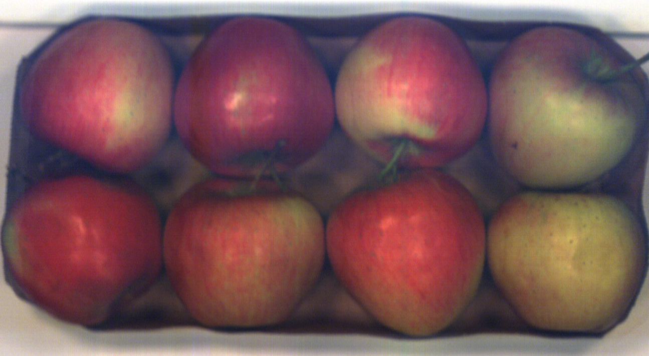
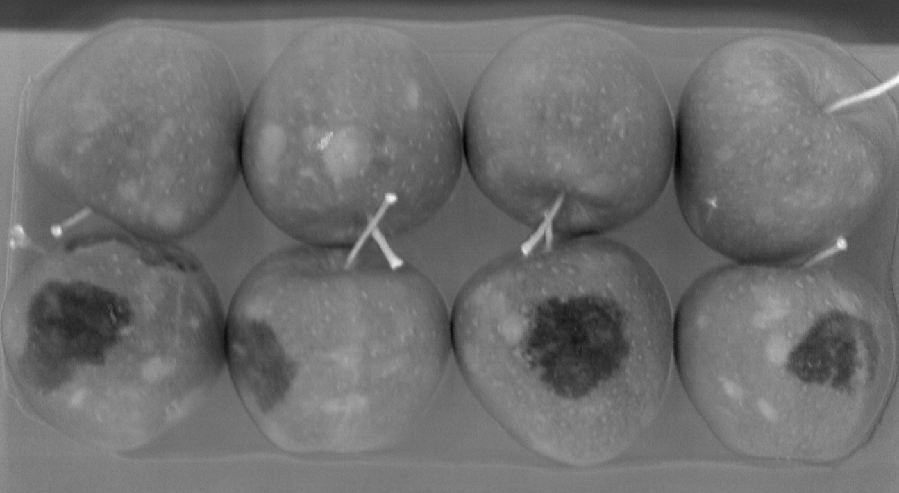
Bruises hidden under apple skin
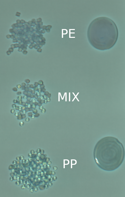
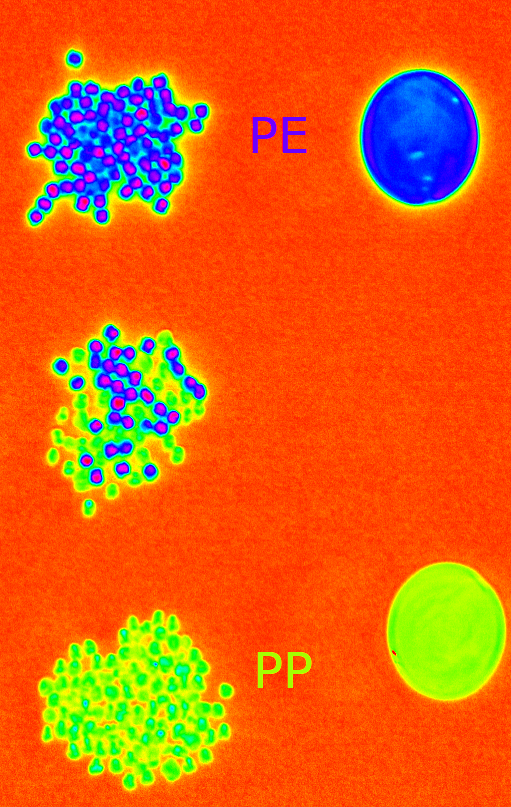
Plastic sorting of polyethylene (PE) and polypropylene (PP) pellets
 Water stress index in olive crops (Human & Physical Geography, CC BY-SA 4.0, via Wikimedia Commons)
Hyperspectral imaging techniques
There are different ways to create hyperspectral images:
- Whisk broom: pixel by pixel scanning using a spectrometer
- Requires either the object or the spectrometer to move in a controlled pattern in order to perform a full scan
- Push broom: line by line scanning using a hyperspectral line sensor
- Requires either the object or the line sensor to move with a fixed speed in order to perform a full scan
- Spectral scanning: sequential capture of the whole subject,
but only a single wavelength at a time
- Requires the object and camera to be static
- Snapshot: a simultaneous full frame scan of all wavelengths
- Allows the object to move but doesn't require it

Push broom
Line by line scanning using a hyperspectral line sensor. Each image output from the sensor represents a full slit spectrum (x, λ), where each line is a wavelength. The images are formed by projecting a strip of the scene onto a slit and dispersing the slit image with a prism or a grating.

It requires either the object or the line sensor to move with a fixed speed in order to perform a full scan. This is typically done by having the object in a conveyor belt.


Intense broadband illumination (e.g. halogen lights) is critical for push broom applications. A big amount of the light intensity is lost through the slit.
Because the detector covers a broad spectral range, higher transmission orders from the diffraction grating become observable, causing overtones. The periodic structure of the grating produces multiple reflection orders, where the zeroth order contains the non-diffracted primary signal, and the higher orders spread the light based on wavelength.
As the detector captures this wide range of wavelengths, the higher orders can spatially overlap with the primary signal, resulting in overtones in the measurement.
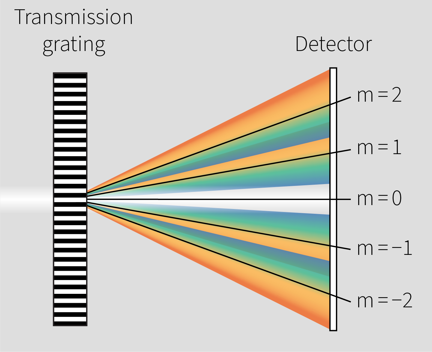
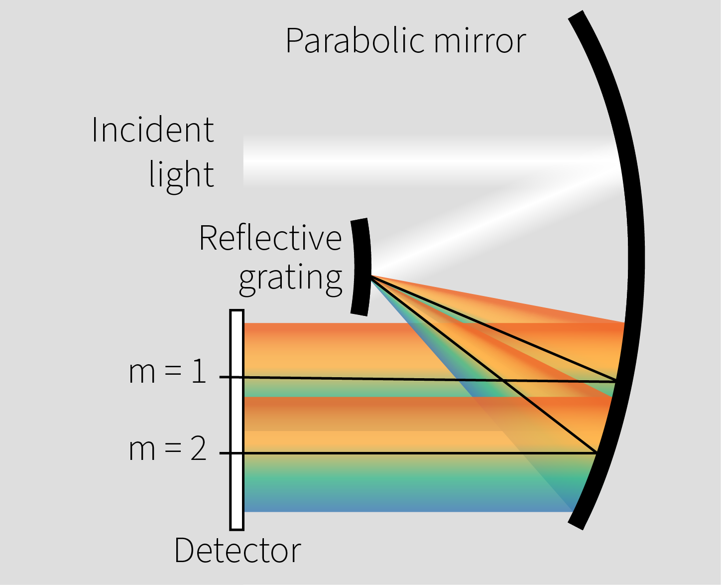
Multiple reflection orders caused by the grating
If necessary these effects can be counteracted by for example adding an external long-pass filter in front of the optics to limit the spectral range. It effectively removes the visible part of the spectrum and with it the overtones that it causes in the infrared range.
Another similar option is to add a long-pass filter internally, covering only the bottom part (infrared range) of the sensor, in order to filter the visible range overtones.
However, all of these methods will result in a decrease of the signal to noise ratio and are therefore up to the user to decide.
Snapshot
A simultaneous full frame scan of all wavelengths (no scanning of any kind is necessary). Figuratively speaking, a single snapshot represents a perspective projection of the datacube, from which its three-dimensional structure can be reconstructed. Can be achieved using different techniques, for example computed tomographic imaging spectrometry (CTIS). The techniques are generally computationally expensive and require dedicated hardware for processing the datacube projection.
This approach has the advantage of not requiring object movement nor it is disturbed by movement. It also generally requires less light than a push-broom camera.
However, the benefits come at the cost of other parameters: for example reduced spectral and/or spatial resolutions, limited spectral range, etc. And the data reconstruction algorithms might also need to be tweaked depending on the specific application.
 Optical layout and reconstruction of CTIS image
 Formation of a CTIS image (ElkoSoltius, CC BY-SA 4.0, via Wikimedia Commons)
Data Cube
The images captured by the hyperspectral sensors are combined into a three-dimensional (x, y, λ) data cube for processing and analysis, where x and y represent two spatial dimensions of the scene, and λ represents the spectral dimension (comprising a range of wavelengths).

File formats
PAM PAM
- "Extension" of the Netpbm file formats
- Simple and very easy to parse
- ASCII header followed by RAW data
- the RAW data is by definition stored as a sequence of tuples (BIP)
- Can also contains multiple images (BSQ)
- No open-source standard viewer (see pam-viewer and/or hsi-viewer)
Example header:
P7
WIDTH 227
HEIGHT 149
DEPTH 3
MAXVAL 255
TUPLTYPE RGB
ENDHDR
ENVI ENVI
- Used as a somewhat "standard" for HSI images
- ASCII header and RAW data in separate files
- the header has some required and many optional fields
- Supports the 3 different interleave types
- No open-source standard viewer (see hsi-viewer)
Required header fields
| Field | Description |
|---|---|
| bands | number of bands per image file |
| byte order | order of the bytes (0: LSF, 1: MSF) |
| data type | type of data representation (1: uint8, 2: int16, 4: float, 5: double, 12: uint16, ...) |
| file type | ENVI-defined file type |
| header offset | number of bytes of embedded header information present in the file (default=0) |
| interleave | data ordering (BSQ, BIP, BIL) |
| lines | number of lines per image for each band |
| samples | number of samples (pixels) per image line for each band |
Example header:
ENVI
description = {
  Registration Result. Method1st degree Polynomial w/ nearest neighbor [Wed Dec 20 23:59:19 1995] }
samples = 709
lines   = 946
bands   = 7
header offset = 0
file type = ENVI Standard
data type = 1
interleave = bsq
sensor type = Landsat TM
byte order = 0
map info = {UTM, 1, 1, 295380.000, 4763640.000, 30.000000, 30.000000, 13, North}
z plot range = {0.00, 255.00}
z plot titles = {Wavelength, Reflectance}
pixel size = {30.000000, 30.000000}
default stretch = 5.0% linear
band names = {
 Warp (Band 1:rs_tm.img), Warp (Band 2:rs_tm.img), Warp (Band 3:rs_tm.img), Warp (Band 4:rs_tm.img), Warp (Band 5:rs_tm.img), Warp (Band 6:rs_tm.img), Warp (Band 7:rs_tm.img)}
wavelength = {
  0.485000,  0.560000,  0.660000,  0.830000,  1.650000, 11.400000,  2.215000}
fwhm = {
 0.070000, 0.080000, 0.060000, 0.140000, 0.200000, 2.100000, 0.270000}
TIFF
- Multiple images (multipage)
- BSQ data ordering
- Can be loaded in image processing programs like ImageJ image-j for processing (using image stacks)
Data ordering
Interleave type of the binary stream of bytes.
Band Sequential (BSQ)
- Each line of the data is followed immediately by the next line in the same spectral band.
- Optimal for spatial (x,y) access of any part of a single spectral band.
- Essentially a sequence of single channel images.
Band-interleaved-by-pixel (BIP)
- Stores the first pixel for all bands in sequential order, followed by the second pixel for all bands, followed by the third pixel for all bands, and so forth, interleaved up to the number of pixels.
- Optimum performance for spectral (z) access of the image data.
- Native data ordering in the PAM format.
Band-interleaved-by-line (BIL)
- Stores the first line of the first band, followed by the first line of the second band, followed by the first line of the third band, interleaved up to the number of bands. Subsequent lines for each band are interleaved in similar fashion.
- Provides a compromise in performance between spatial and spectral processing.
- "Native" format on the sensor for push-broom cameras.
Data processing
Useful methods for pre/post processing and visualizing HSI data.
Reflectance model
Transforming the RAW data into a reflectance model is a very useful (and borderline crucial) pre-processing step when handling hyperspectral data.
It will make the resulting data a lot more robust by reducing pixel intensity differences caused by different internal and external factors. One of the relevant external factors is variations in the illumination: either between sample acquisitions (in the same or different systems) or simply because of uneven lighting conditions through the field of view. An internal factor is for example response curve differences between different cameras and even internal differences between pixel responses in the image sensor itself (and defective pixels). Therefore the resulting data will be a lot more suitable for use in generating classification models (specially when training AI based models).
This can be done by acquiring both a black and a white reference images.
Black reference
The black reference image is acquired by putting a lens cap on, blocking all light from the sensor. The black reference is used to model the dark current in the sensor and can also show the position of "hot pixels" (which are a kind of defective pixel which appears bright in the black reference) so that they can be later corrected.
White reference
The white reference image is acquired by placing a reference plate under the camera covering the entire field of view. The reference plate must be made from a material which is uniformly reflective through the whole relevant spectrum. The white reference focus mostly on modeling the illumination and the sensor response to it. It will compensate for both spacial and spectral non-uniformities caused by the light source. Moreover, it will also compensate for differences in the sensor spectral response to the different light wavelengths and for differences in the pixel responses through the sensor. Finally, the white reference will also show the position of "dead pixels" (which are a kind of defective pixel which appears dark in the white reference) so that they can be later corrected.
When acquiring a white reference image it is important to maximize it's response while avoiding saturation, by adjusting the exposure time. However, if the sample to be measured is a lot darker than the white reference, then the signal-to-noise ratio (SNR) might not be optimal on the sample itself. In that case it can be an advantage to use a grey reference instead of a white one. Or to make the captures with two different exposure times: a lower one for the white reference and a higher one for the sample, and then compensate afterwards.
RESTAN restan (reflection standard) is one of the materials we recommend for white reference plates since it diffusely reflects more than 98% of light in the area between 300nm and 1700nm.
It is also possible to use TiO2 (Titanium dioxide) or BaSO4 (Barium sulfate) in powder form, though their reflectance is not as high or uniform as RESTAN, which is PTFE (Polytetrafluoroethylene) based.
Conversion to reflectance
In order to create a reflectance model from the RAW data it is necessary to subtract the black reference and then divide by the difference between the white and the black references:
No image sensor is completely perfect: they all contain some small amount of imperfect pixels which generally need to be taken into account when analyzing images since they will have very poor signal-to-noise ratio (SNR). This is even more critical when doing the conversion to the reflectance model because they can result in divisions by zero (or very small numbers).
The imperfect pixels can for example be "dead" (or with lower than expected response), which can be seen on the white reference or "hot" (with brighter than expected response), which can be seen on the dark reference. And they will generally have very similar values in both the black and white references.
Defective pixels can be simply ignored (skipped over) or alternatively "compensated" for by for example using a median filter of suitable size at their position.
Re-calibration
In some cases (laboratory use) it is easy to acquire new black and white references for every sample, and that guarantees the most robust results. This is however not feasible in an industrial environment (e.g. production lines).
Therefore, since the black reference function is to compensate for the dark current, it can be sufficient to acquire a new reference only when factors related to the dark current change: for example exposure time, image size (cropping) and ambient temperature (for sensors which aren't actively cooled or temperature compensated).
Likewise, since the white reference depends on the illumination and sensor response, it can be sufficient to acquire a new reference only when parameters related to these factors change: for example exposure time and lighting conditions (including ambient light).
But it is still recommended to do some sort of periodical (e.g. once a month) "re-calibration" by acquiring new reference images.
Filtering
Imperfections in the sensor itself (see "dead/hot pixels" above) or in the spectrograph (e.g. slit) can result in artifacts in the image (e.g. lines). Moreover, depending on for example the illumination available and the sensor spectral response curve, the signal-to-noise ratio (SNR) might not be optimal through the whole data cube.
Therefore, another possibly beneficial pre-processing step is to apply some noise filtering to the RAW data. For example a small gaussian filter can be used.
Data visualization and "false" coloring
There are different ways to inspect the data from the data cube: for example looking at full monochrome images of single spectral bands (or averaging neighboring bands into one) or by plotting the graph of the full spectral response of a specific spatial region.
The monochrome images can have color maps applied to it in order to make the intensity differences more prominent.
Moreover, in many cases, it can also be useful to construct "false" RGB images using the input data. The simplest option is to create an actual RGB representation by selecting the appropriate wavelengths for red (~600-700nm), green (~500-600nm) and blue (~400-500nm).
Another option which can be useful when infrared data is present is generating a Color-Infrared Image. A CIR image is created by basically shifting the RGB colors so that infrared (IR) is rendered as RED, red is shown as GREEN and green is shown as BLUE. The input blue wavelengths get shifted out and appear as black.

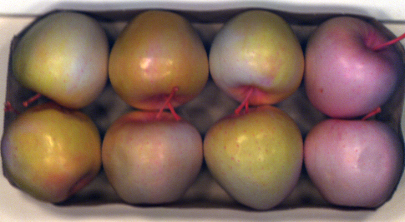
RGB (left) and CIR (right) representations of apples datacube
CIR images are widely used for maps with vegetation present. In CIR images dense vegetation (with a lot of chlorophyll) will generally appear as bright red, while less dense vegetation (less chlorophyll) will have lighter tones of red, magenta or pink. Dead and unhealthy plants can present in green or tan. White, blue, green and tan will often represent soil, with darker shades possibly indicating higher moisture levels. Buildings and roads tend to appear white or light blue. Water might show as dark blue or black.
For both the RGB and CIR cases it is possible to select single spectral bands or to average the results over several bands (which can provide some noise reduction).
Spectral band math
One of the simplest ways to isolate and enhance specific features/objects in the images is to look for prominent differences in specific spectral bands. Then simple arithmetic operations (addition, subtraction, multiplication, division, ...) can be performed using the images containing these specific spectral bands.
Example
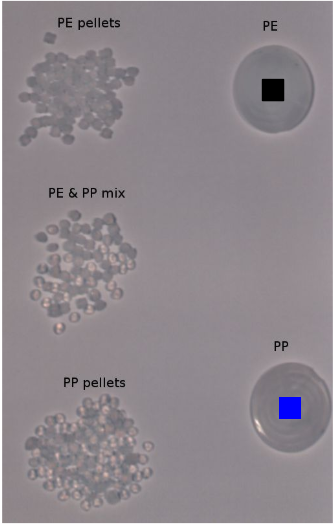
Simple plastic sorting of polyethylene (PE) and polypropylene (PP) pellets.


Polyethylene (PE) and polypropylene (PP) pellets: PE (top), PE+PP mix (middle), PP (bottom)
- Analyze spectral bands and identify bands with big spectral differences.

Montage of spectral bands of polyethylene (PE) and polypropylene (PP) pellets.
Created by loading a TIFF data cube into ImageJ and choosing: Image → Stacks → Make Montage.
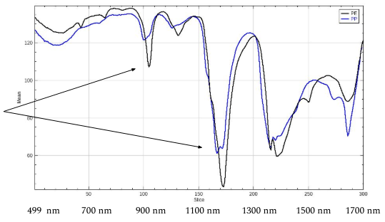
Spectral bands of PE and PP plastic, showing regions with big differences.
Created by loading a TIFF data cube into ImageJ and choosing: Image → Stacks → Plot Z-profile.
The graph above clearly shows big differences between the 2 types of plastics at some specific wavelengths (e.g. ~920nm and ~1200nm). Which means it could be possible to differentiate between the PE and PP by using simple band math.
If for example bands 168 (~1172nm) and 174 (~1196nm) are subtracted from each other:

PE and PP plastic classification by subtraction of spectral bands: 168 (~1172nm) and 174 (~1196nm)
- Resulting image: I = band 168 - band 174
- If I < -2.5 → PP
- If I > 13.5 → PE
Dimensionality reduction
Due to the large amount of data present in hyperspectral images it can be highly beneficial to apply techniques which reduce the resulting amount of data by transforming the input data in order to maximize the variation.
Examples of such techniques are principal component analysis (PCA) and partial least squares (PLS) regression.
Principal component analysis (PCA)
Principal component analysis (PCA) is a linear dimensionality reduction technique with applications in exploratory data analysis, visualization and data preprocessing.
The data is linearly transformed onto a new coordinate system such that the directions (principal components) capturing the largest variation in the data can be easily identified. The 1st component captures the most variance, the 2nd captures the next most, and so on. Therefore it can greatly reduce the number of dimensions (channels) in a datacube while preserving as much information as possible.
Moreover it means that if the original data has a high degree of correlation between its spectral bands then only a few principal components are sufficient to describe most of the data variance.
The most basic usage of PCA is for example to separate the objects from the background (which is normally visible in the first couple of components).

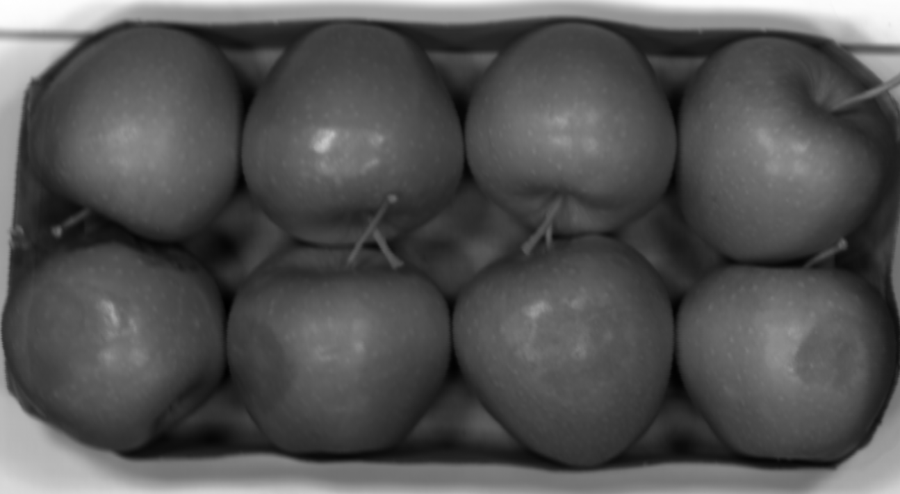
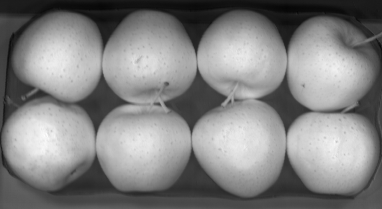
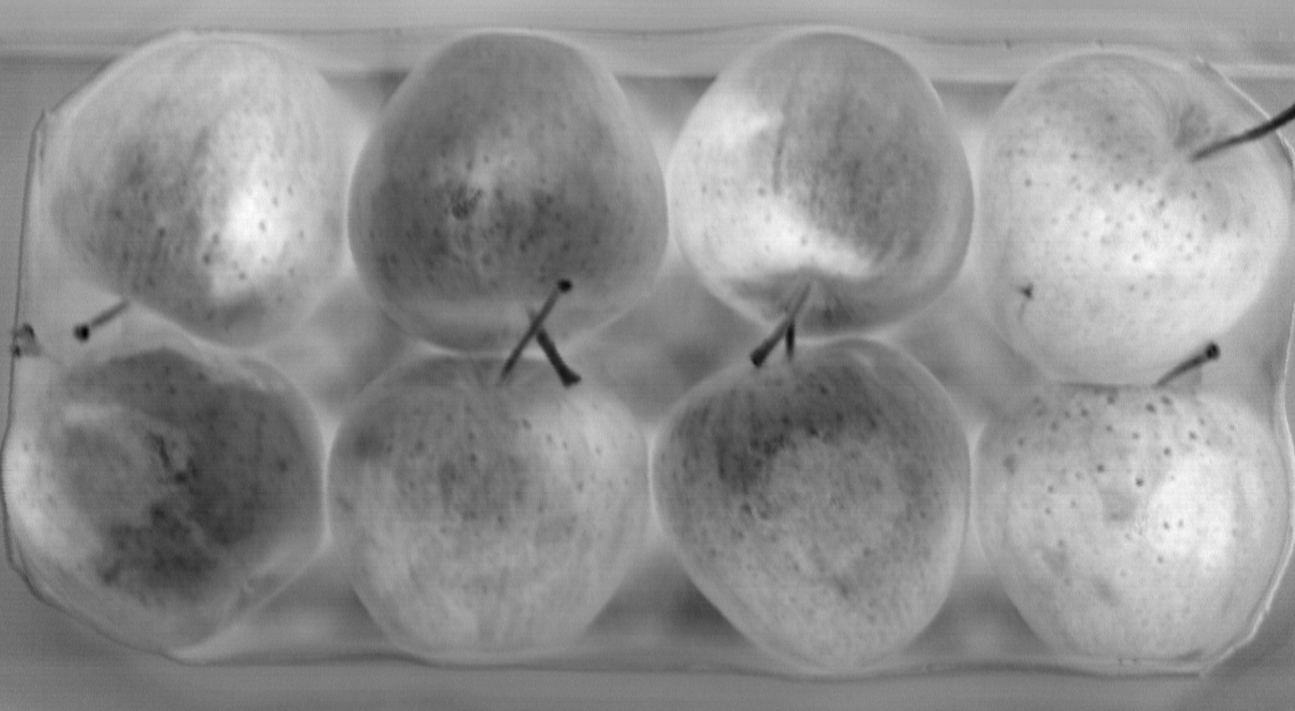
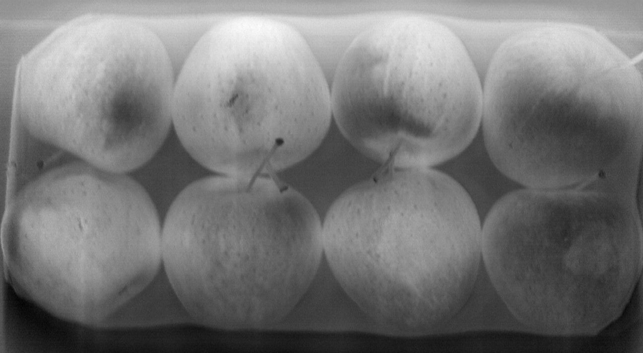
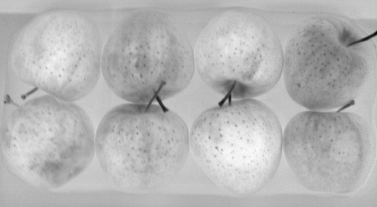
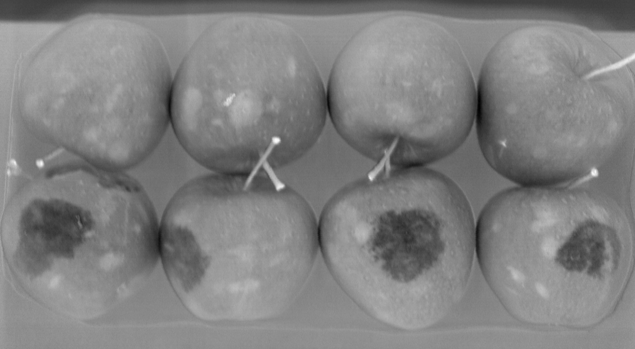
PCA with 6 components on apple HSI image
The example above shows that the 1st PCA component separates the apple tray from it's surroundings, while the 2nd PCA component can easily be used to segment the apples themselves from the background. The other PCA components highlight different details of the image. For example the 6th component highlights the bruises under the apples skin, while the 5th component highlights details on the skin itself. Other components might be focusing on the visible color differences in the different areas. Higher level PCA components were excluded since they highlighted only the noise present in the data cube, meaning that there was no more relevant variance in the data.
Band selection/reduction
The PCA also provides information about the contribution (positive or negative) of each channel to each component. In this way it is possible to determine which spectral bands contribute the most to each principal component, which can be used to do band selection (reduce the amount of input spectral bands on the camera in order to speed up image capture and processing).

Contributions of each spectral band to the 6 principal components of the apple example above
Partial least squares (PLS) regression
Partial least squares regression (PLS) is a statistical method that bears some relation to principal components regression. But instead of finding hyperplanes of maximum variance between the response and independent variables, it finds a linear regression model by projecting the predicted variables and the observable variables to a new space. Because both the X and Y data are projected to new spaces, the PLS family of methods are known as bilinear factor models.
Partial least squares discriminant analysis (PLS-DA) is a variant used when the Y is categorical, which is useful for classifying objects into groups.
AI models
When the problem is too complex and the simpler methods fail a good option might be to train AI models instead.
The big downside of this method is that it generally requires a big amount of input data (which normally needs to be annotated and with enough variation) in order to be robust (~100-1000+ samples). Moreover, it can be hard to predict how the models will react to "new" (previously unseen) inputs since the resulting "algorithm" is mostly a "black box".
Visualization/processing tools
As mentioned above the aren't any standard open source tools for hyperspectral data visualization and processing. Therefore qtec has developed it's own tools (hsi-viewer) for data cube visualization and some basic data processing.
Qtec has also a partnership with Prediktera which develops advanced tools for hyperspectral data capture and processing (license based).
hsi-viewer
- Helper tool developed by qtec for visualizing and manipulating HSI data cubes.
- Supports importing/exporting PAM, ENVI and TIFF file formats.
- Shows individual slices of the cube (full images in a single selectable spectral band) with color maps.
- Can plot the mean spectra of rectangular regions of the images for comparison.
- Optional SNV (Standard Normal Variate) for spectra normalization
- Spectral derivatives
- Optional smoothing (Gaussian, Savitzky Golay)
- Supports opening and comparing multiple images at a time.
- Efficient data loading to minimize RAM usage.
- Compose false "RGB" image from selected bands.
- Also handles reflectance calibration (using white/black references).
- PCA (under development)
- Python based.
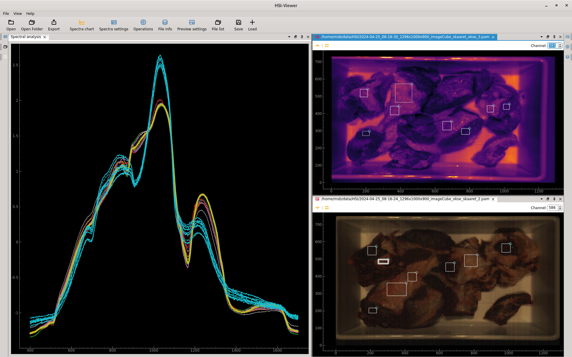
hsi-viewer showing spectral curve of meat and fat regions
The hsi-viewer is still under development.
Availability of an alpha version for testing is expected soon.
Prediktera prediktera
Prediktera provides state of the art software for research, application development and real-time analysis. It is a complete software toolset for hyperspectral imaging.
Prediktera Breeze is a complete solution for hyperspectral data analysis and creation of real-time data processing applications. Breeze requires no programming experience and includes many widely used HSI processing methods as well as advanced machine learning algorithms.

The following software packages are available through licenses (yearly or perpetual):
- Evince: Explore Hyperspectral Imaging
- Breeze: Develop and Run Applications
- Breeze runtime: Integrated Realtime Solutions
Prediktera offers 30 day trials of their software.
Prediktera offers an interface for qtec's Hypervision 1700 cameras in their software suite starting from release 2024.3 (November 2024).
Qtec HSI Cameras
Qtec currently offers two versions of push-broom hyperspectral cameras, named Hypervision.
The Hypervision cameras are of push-broom (line-scan) type and cover either the VIS-NIR (430-1000nm) or the VIS-SWIR (430-1700nm) ranges, with up to 900 spectral bands.
We are also currently developing a second type of camera using the CTIS principle. The CTIS camera is a snapshot ("full frame") hyperspectral camera which operates in part of the VIS-NIR range (600-850nm), with up to 145 spectral bands.
| Hypervision 1000 | Hypervision 1700 | CTIS* | |
|---|---|---|---|
| Type | push-broom | push-broom | snapshot |
| Wavelength range | 430-1000 nm | 430-1700nm | 600-850nm |
| Spectral bands | 330 | 900 | 145 |
| Rayleigh resolution (w. 10um slit) | 3.9 nm | 3.9nm | NA |
| Spectral resolution | 1.77 nm/px | 1.5 nm/px | 1.72 nm |
| ROI (band selection) | individual band selection | 8x vertical groups | None |
| Spatial resolution | 1840 px | 1280 px | 312 x 312 px |
| Pixel size | 6.5 um | 5 um | 6.5 um |
| Maximum framerate* | 250 fps | 150 fps | 40 fps (89) |
Measured with all spectral bands selected.
The push-broom type cameras can achieve a much higher framerate if less spectral bands are selected through regions of interest (ROI).
The CTIS type camera can achieve higher capture speeds (up to 89 fps), but is limited to 40 fps because of the cube reconstruction speed.
The CTIS camera is still under development and is therefore currently not available for purchase.
Hypervision
Refer to the Hypervision HSI Cameras section for more information.

CTIS
Qtec's Snapshot hyperspectral camera.

It produces a full frame image with up to 145 spectral bands. It covers both the red and part of the near-infrared spectrums (600-850nm range). The wavelengths were chosen with focus on agricultural applications.
The reconstruction of the data cube from the projections on the input image is AI driven (requires hailo module) and might need to be tweaked depending on the specific application.
| CTIS | |
|---|---|
| Wavelength range | 600-850 nm |
| Spectral bands | 145 |
| Spectral resolution | 1.72 nm |
| Spatial resolution | 312 x 312 px |
| Pixel size | 6.5 um |
| Maximum framerate* | 40 fps (89) |
The camera can achieve higher capture speeds (up to 89 fps), but is limited to 40 fps because of the cube reconstruction speed.
The big advantage of this camera is being able to make an instantaneous full frame scan of an object (and it also requires much less light that the Oculus cameras), which makes it more flexible for usage in field applications. However, the benefits come at the cost of reduced spatial resolution and a more limited spectral range.
The CTIS camera is still under development and is therefore currently not available for purchase.