HV Explorer
Python based helper tool developed by qtec for visualizing and manipulating HSI data cubes.
Features
It supports importing and exporting to/from difference datacube file formats (currently PAM, ENVI and TIFF). The data can then be visualized as individual slices of the cube shown as full images (of a single selectable spectral band) with different color maps or by composing false "RGB" image from selected bands.
Moreover, it can also plot the mean spectra of multiple rectangular regions of the images for comparison. The spectra can then, if desired, be normalized using SNV (Standard Normal Variate) and/or smoothed (using Gaussian or Savitzky Golay smoothing methods). Optionally, the spectral derivatives (1st or 2nd orders) can be plotted. The spectra of the selected regions can be exported in the CSV format.
Multiple images can be opened and compared at once due to HV SDK's efficient data loading which minimizes RAM usage (Buteo data cubes are often 1Gbyte in size which can overload normal programs).
The HV Explorer supports several common HSI image transformations, including reflectance calibration (using white/black references), dimensionality reduction (PCA), clustering, noise reduction, dead pixel removal, band math, etc.
The HV Explorer currently requires the datacubes to be have been captured beforehand through the Buteo Hyperspectral Imaging System interface (or by other means), but support for capturing live data directly from the Hypervision cameras will be added in subsequent releases.
Both Linux and Windows versions are available.
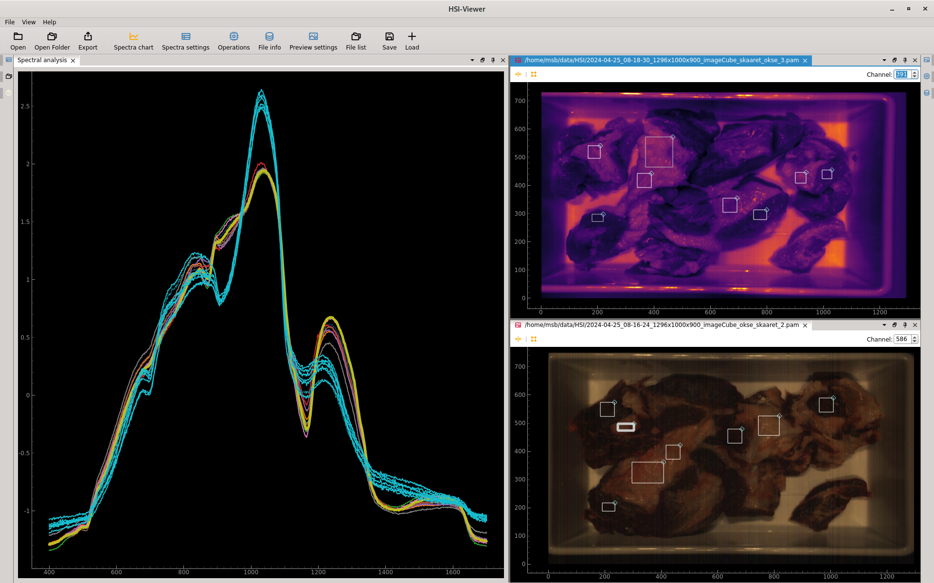
HV Explorer showing spectral curve of meat and fat regions
The HV Explorer is still under development.
The alpha version has been released in March 2025 and the next release will include some classification tools. Live data capture support is expected by the end of 2025.
Some features such as dead pixel removal and band math are still not fully implemented and will be added in subsequent releases.
Windows11 or Linux (Python 3.10 or higher required)
Minimum RAM: 8Gb (16Gb recommended)
Installation
Windows
Simply download the latest Qtec-HV-Explorer-Setup.exe
and follow the instructions.
Linux
installation script
The installation script automatically performs all the steps described below in the uv section.
You can use curl to download the script and execute it with bash:
curl -LsSf https://gitlab.com/api/v4/projects/67863505/packages/generic/qtec-hv-explorer/0.2.3/install.sh | bash
If your system doesn't have curl, you can use wget:
wget -qO- https://gitlab.com/api/v4/projects/67863505/packages/generic/qtec-hv-explorer/0.2.3/install.sh | bash
uv
uv can install/update the package directly from the repository. You need to have the tool installed, then run:
uv tool install qtec-hv-explorer@0.2.3 --index https://gitlab.com/api/v4/projects/67863505/packages/pypi/simple --index-strategy unsafe-best-match --prerelease=allow
To create an application shortcut, copy HV-Explorer.desktop
and hv-explorer.svg
to the appropriate locations or use the example commands below:
cp <download_path>/HV-Explorer.desktop ~/.local/share/applications/
sudo cp <download_path>/hv-explorer.svg /usr/share/icons/
Tutorial
This tutorial was generated based on the HV Explorer version 0.2.3
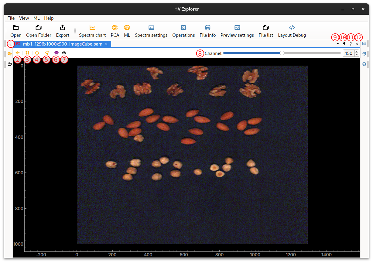
Start by opening the HV Explorer, the following interface will be appear:
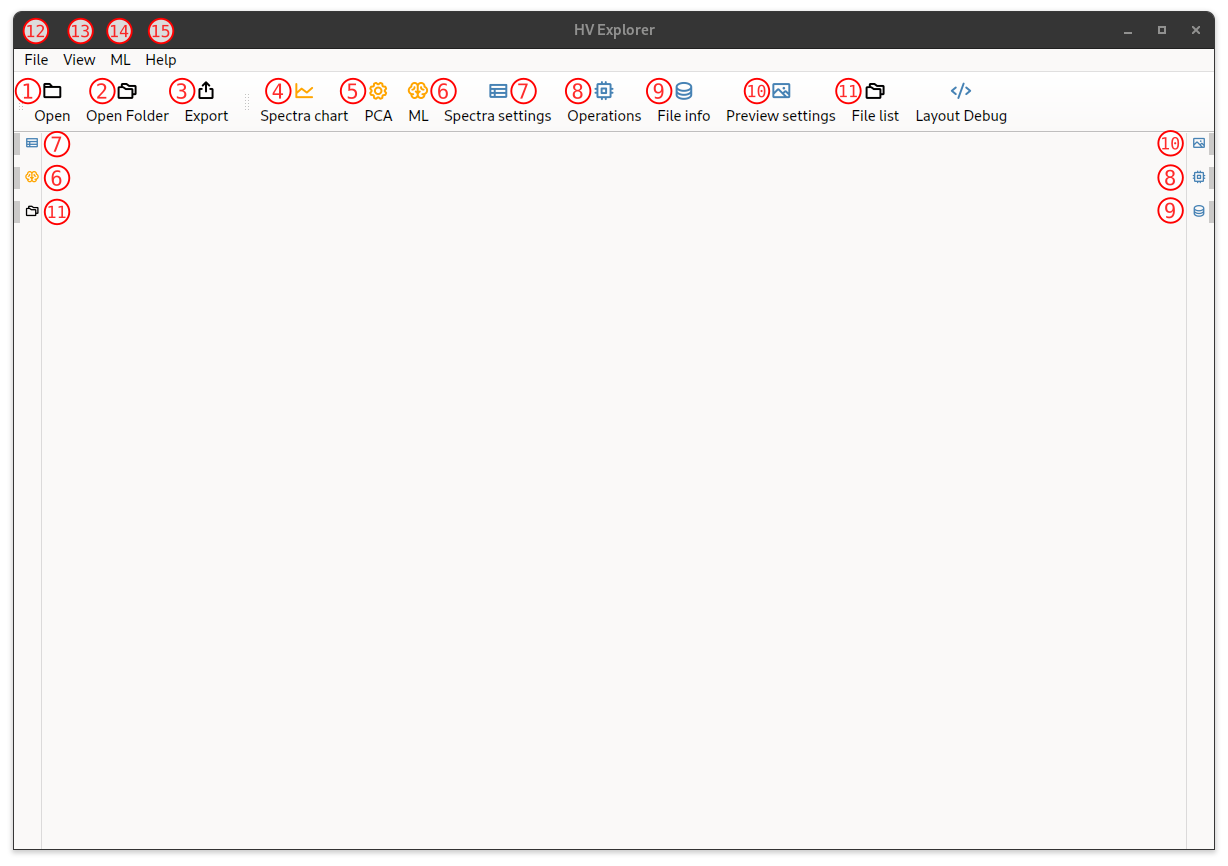
HV Explorer interface
| Number | Name | Description |
|---|---|---|
| 1 | Open file | Opens a file containig a datacube Supported formats: PAM, ENVI (HDR) and TIFF |
| 2 | Open folder | Sets the "root folder" for the "File list (11)" |
| 3 | Export | Exports the resulting datacube (after the selected operations have been applied) Supported formats:PAM, ENVI (HDR) and TIFF Supported interleave types: BIL, BIP and BSQ |
| 4 | Spectra chart | Shows the plot containing all the selected spectra (average spectrum from each ROI) |
| 5 | PCA | Runs a PCA based on the ROIs and shows the plot of the result (can select the compenent for each axis) |
| 6 | ML | Shows the interface for training ML models based on the ROIs |
| 7 | Spectra settings | Shows the interface for configuring the "Spectra chart (4)": name the ROIs, hide/show ROIs, select ROI color, create/assign properties to data, apply filters, ... |
| 8 | Operations | Shows the interface for appliying operations to the datacube: calibration, crop, binning, band selection, apply ML models, ... |
| 9 | File info | Shows information about the datacube: Interleave type, shape, data type, wavelengths, ... |
| 10 | Preview settings | Shows the interface for configuring the datacube preview options: false RGB (select bands) or specific band with color map |
| 11 | File list | File explorer interface Defaults to home, change with "Open folder (2)" |
| 12 | File menu | Operations related to files: "Open file (1)", "Open folder (2)" and "Export" |
| 13 | View menu | Operations related to visualization: "Spectra chart (4), "PCA (5)" and "ML (6)" |
| 14 | ML menu | |
| 15 | Help | About HV Explorer (version and copyright) License information |
Example data
Qtec provides some example datacubes for testing the HV Explorer.
The datacubes where captured using the Buteo Hyperspectral Imaging System.
Loading datacubes
Click on the File list (11) icon on the left side, and navigate to the
folder containing the datacube to be loaded.
By default the File list starts in the home directory, but this can be
changed using the Open folder (2) dialog.
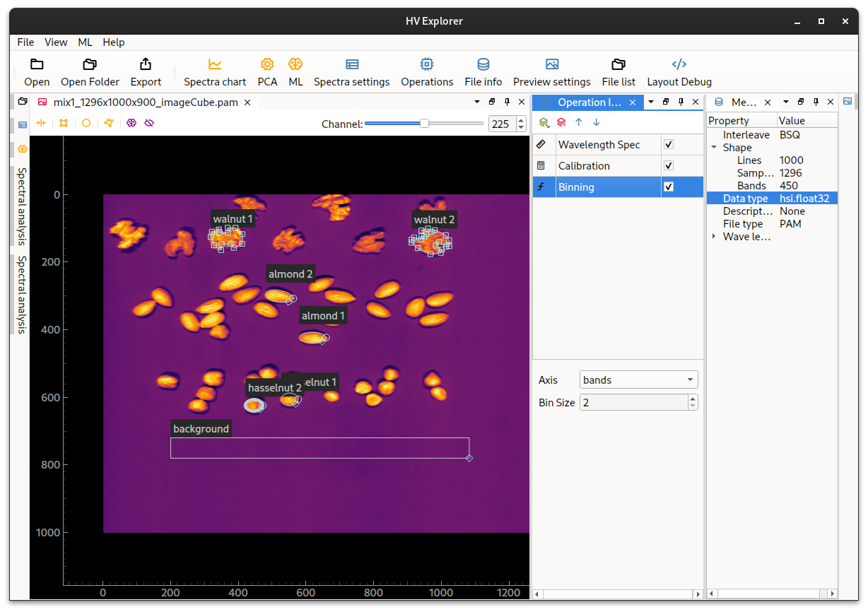
In this example we have used the mixed nuts example data: mix1_1296x1000x900_imageCube.pam, containing almonds, walnuts and hasselnuts.
Alternatively use the Open (1) button on the tool bar at the top to get a
"file dialog".
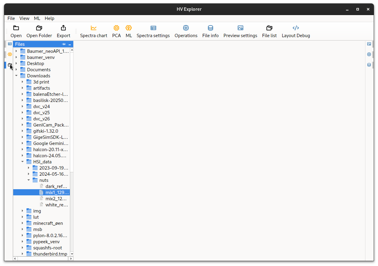
HV Explorer: file explorer interface
The datacube will be loaded.
By default an image of the "middle" band of the cube will be shown (in this
case the cube has 900 bands so band 450 is shown).
An inferno color map is used by default (color maps help enhance contrast in order
to aid the visualization of grey scale data).
It is possible to move the image around and zoom in/out by using the mouse.
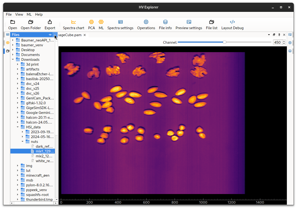
HV Explorer: image loaded
The File list can be minimized by clicking on the "minimize" button (on the
top right corner).
Demo
HV Explorer: loading datacubes
Note that HV SDK (the HV Explorer backend) supports
all three types of interleave for the
PAM file format.
However, in order to determine the interleave and properly load the files, it
expects the interleave type to be specified in the TUPLTYPE part of the header.
File View
HV Explorer: file view interface
| Number | Name | Description |
|---|---|---|
| 1 | File name | Name of the datacube |
| 2 | Slice | Show a slice of the datacube The slice position can be selected |
| 3 | Rectangular ROI | Create a rectangular ROI for averaging the spectra (which will be displayed in the Spectra chart) Size and position can be adjusted |
| 4 | Elliptical ROI | Create an elliptical ROI for averaging the spectra (which will be displayed in the Spectra chart) Size, position and angle can be adjusted |
| 5 | Polygonal ROI | Create a polygon based ROI for averaging the spectra (which will be displayed in the Spectra chart) Created by selecting multiple points |
| 6 | ML model selection | Choose ML model to generate the overlay |
| 7 | Overlay | Enable/disable overlay of result from ML model |
| 8 | Channel/band selection | Select which channel/band is being shown |
| 9 | List all tabs | |
| 10 | Dettach group | Make the current interface "float", so that it can be moved around and attached to a new position |
| 11 | Pin active tab | |
| 12 | Close group | Closes the image. Note that the ROIs persist and aren't removed If the file is opened again the original ROIs will be automatically shown |
Preview Inspector
Click on the Preview Inspector (10) icon on the right side in order to change the
preview settings: select a different color map or change the band/channel shown.
It is also possible to change bewteen visualizing the Gray bands/channels or
creating a "false RGB" Color image representation composed of the specified
bands/channels.
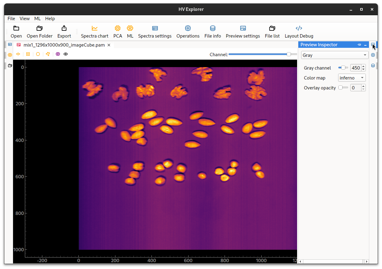
HV Explorer: image preview settings
There are also in-build presets which select the appropriate bands/channels in order to generate a proper RGB visualization of the datacube, however this requires setting up information about the wavelengths covered by the datacube (otherwise the preset option is disabled in the interface).
This can be done by opening the Operation Inspector (8) icon on the right side.
Then click the "plus" icon in order to add a new operation and choose the
WavelengthSpec operation.
Now type in the start and end wavelengths for the datacube, in this example the
data was captured using a
Hypervision 1700
camera with all bands present, so the minimum wavelength is 430nm and the maximum
wavelength is 1700nm.

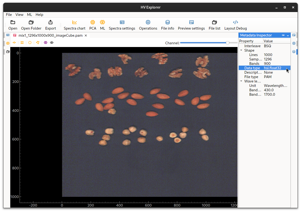
HV Explorer: wavelength information
This information is now available in the File info / Metadata inspector (9),
along with image dimensions (lines, samples and bands),
interleave type and data type
((un)signed integer/float with 8, 16, 32 or 64 bits).
The image dimensions are defined as:
- lines: number of raw images, corresponding to "image height"
- samples: spatial width
- bands: number of channels/wavelengths
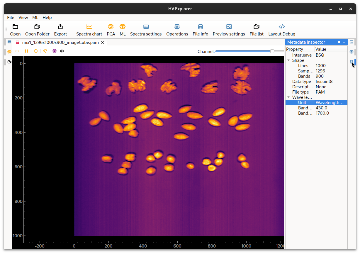
HV Explorer: metadata information
Now a False RGB color preset can be choosen in the Preview Inspector (10).
The bands used for the red, green and blue channels can be changed, if desired, in order to generate a different visual representation of the data.
Note that the generated image doesn't seem to be a good representation of the expected color image, it is too redish, this is due to missing "white balancing", which will be performed in the next step by doing "Reflectance calibration".
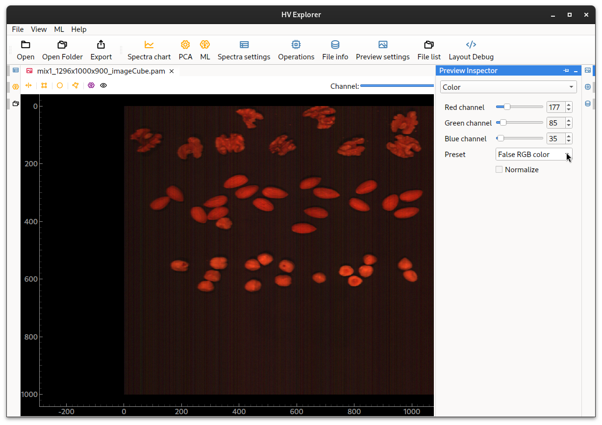
HV Explorer: false RGB color image (missing white balancing)
Alternatively, by choosing Normalize the HV explorer will perform a simple
"white balance" by normalizing the channels, which might improve the false RGB
image without reflectance calibration.
Note however that a lot of noise becomes visible and therefore it is a much better choice (strongly reccomended) to perform the "Reflectance calibration" instead.
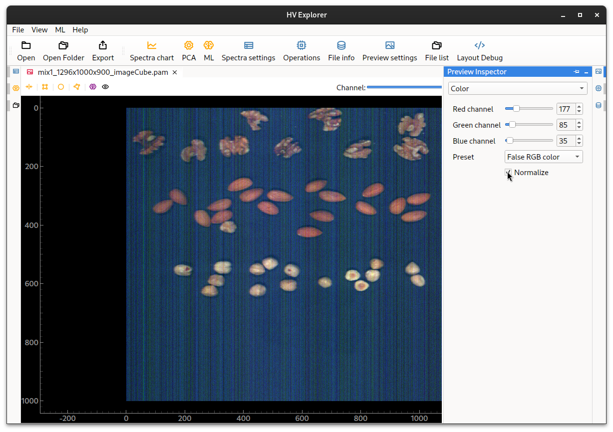
HV Explorer: normalized false RGB color image
Demo
HV Explorer: Preview inspector
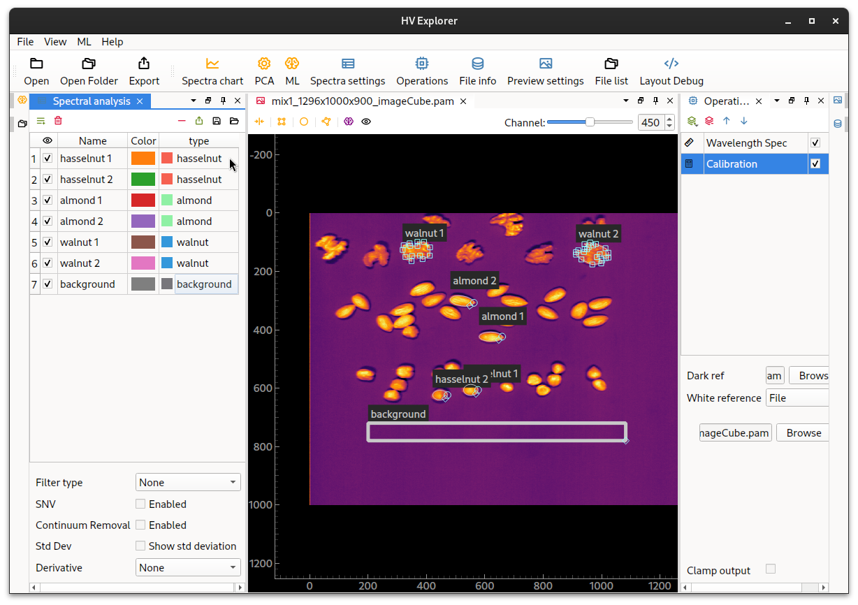
Reflectance calibration
As mentioned above, the color balance of the False RGB image is not correct. This can be adjusted by converting the data into a reflectance model using both a white and a black reference image. The white reference image will adjust the color balance between the different wavelengths as well as correct for differences in illumination through the FOV (field of view). The black reference image will adjust the black level. See the Reflectance model section for in-depth information about the process.
The reflectance calibration can be performed by opening the Operation Inspector (8)
and adding a Calibration operation.
Then selecting the White reference and Dark reference files.
For this example we have used:
- black reference: dark_ref_1296x100x900_imageCube.pam
- white reference: white_ref_1296x100x900_imageCube.pam
Note that is it also possible to use a White Reference which is embedded in
the original datacube by selecting Inline instead of File and then adjusting
the start and end positions of the white target in the image.
The false RGB color image now looks like a more real color representation of the data.

HV Explorer: reflectance calibration (correct false RGB color)
Although it is clearly best to use both a white and a black reference it is possible to apply only one of them to the datacube. Applying the white reference will generally result in a "white balanced" image. While applying the dark reference will help with decreasing noise (specially the vertical lines seen in the Normalized false RGB image).
Scaling
Note that doing a reflectance calibration will transform the data type from the
original unsigned 8-bit integer into a 32-bit float (clipped between 0 and 1).
This can be verified through the Metadata Inspector.
HV Explorer: 32-bit float datatype
Therefore if the new datacube (reflectance calibrated) is to be exported into, for example PAM, it has to be first converted back into an unsigned integer type of either 8 or 16-bit (since this is what PAM supports).
This can be done using a Scaling operation.
Just selected the desired datatype, in this case 8 or 16-bit unsigned, and then
adjust the Scale to an appropriate value (255 for 8-bit and 65535 for 16-bit).
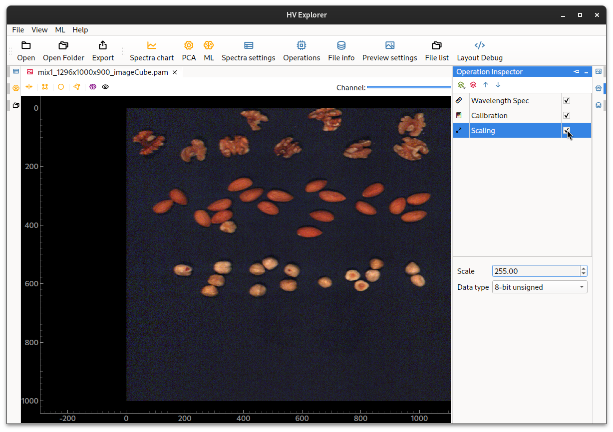
HV Explorer: reflectance calibration (after scaling)
The individual operations can be enabled/disabled by clicking on the checkbox to their right.
Alternatively, they can also be completely removed by clicking on the
Remove operation button (red minus at the top bar).
Demo
HV Explorer: Reflectance calibration
Operation Inspector
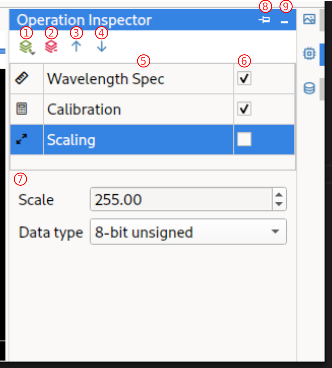
HV Explorer: Operation Inspector interface
| Number | Name | Description |
|---|---|---|
| 1 | Add operation | Add a new operation to the bottom of the list |
| 2 | Remove operation | Remove the selected operation |
| 3 | Move operation up | Move selected operation up (will be applied earlier in the "pipeline") |
| 4 | Move operation down | Move selected operation down (will be applied later in the "pipeline") |
| 5 | Operation list | List of operations with order of execution |
| 6 | Enable/disable operation | Enable/disable specific operation |
| 7 | Operation options | Options related to the specific operation |
| 8 | Pin panel | Pin the panel to graphical interface (so that it is not on top of the image but next to it) |
| 9 | Minimize panel | Hide the Operation Inspector |
The order of the individual operations can be changed by using the up/down arrows
in the Operation Inspector.
However, the Calibration operation should generally be one of the first ones.
Spectral plot
Now we will move into showning how to plot spectral information.
Choose one of the ROI options from the File View (rectangular,
elliptical or polygonal).
For example, click on the elliptical spectrum icon on the top of the image.
This will add an elliptical selection box to the middle of the image.
Move, resize and angle the ellipse as desired in order to select the region from which spectral data is desired (the data inside the ROI will be averaged). Add as many selection areas as desired.
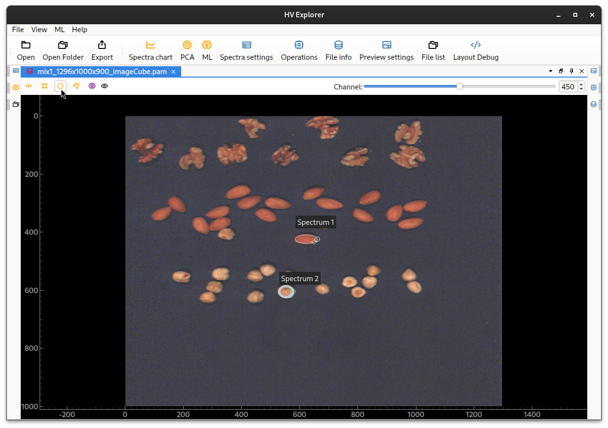
HV Explorer: ROI selection placement
When using the polygonal ROI tool, click to create consecutive point segments.
Close the selection area (polygon) by either pressing the ENTER key on the
keyboard or clicking on the first point of the segment.
Note that points can be later added/removed from the polygon, as well as moved around. To add new points click on a line segment of the polygon. To remove points right click on a point and select remove handle.

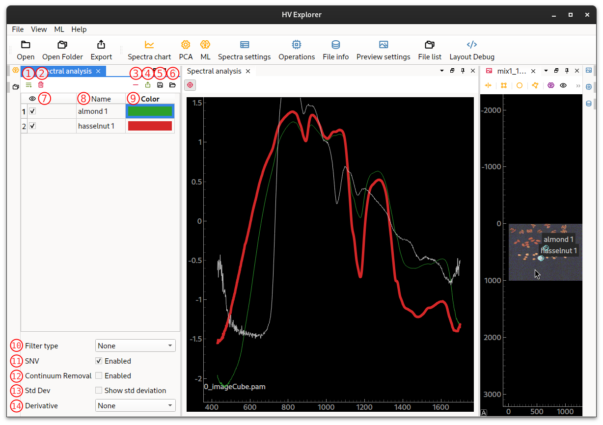
Now open the Spectral settings (7) panel on the left.
A list of the created selection areas is displayed, each with a color and a name.
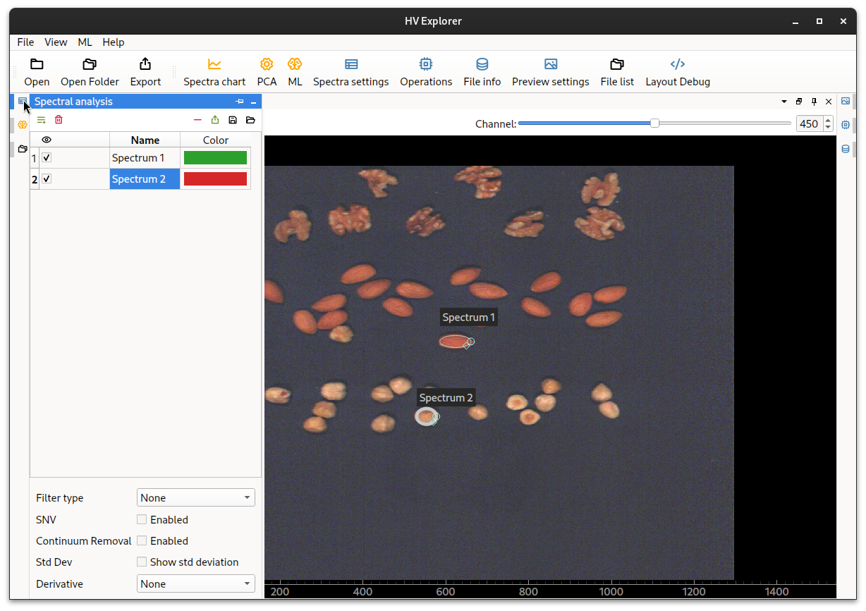
HV Explorer: Spectral analysis panel
Change the names and colors as necessary by double clicking.
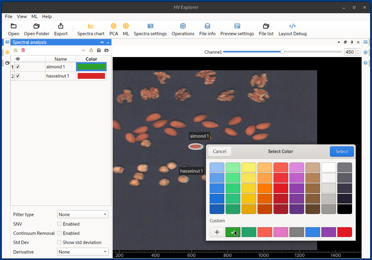
HV Explorer: spectra color picker
Now click on the Spectral chart (4) icon on the tool bar at the top.
This will open a plot view for the spectral data contained in the selection areas.
Clicking on the different spectra inside the Spectral analysis panel will
"highlight" both the selected spectra in the Spectral chart plot as well as
the corresponding selection area in the image.
It is possible to remove a selection box from the image (and therefore removing
the corresponding data from the plot) by selecting it in the Spectral analysis
panel and then clicking on the red minus icon.
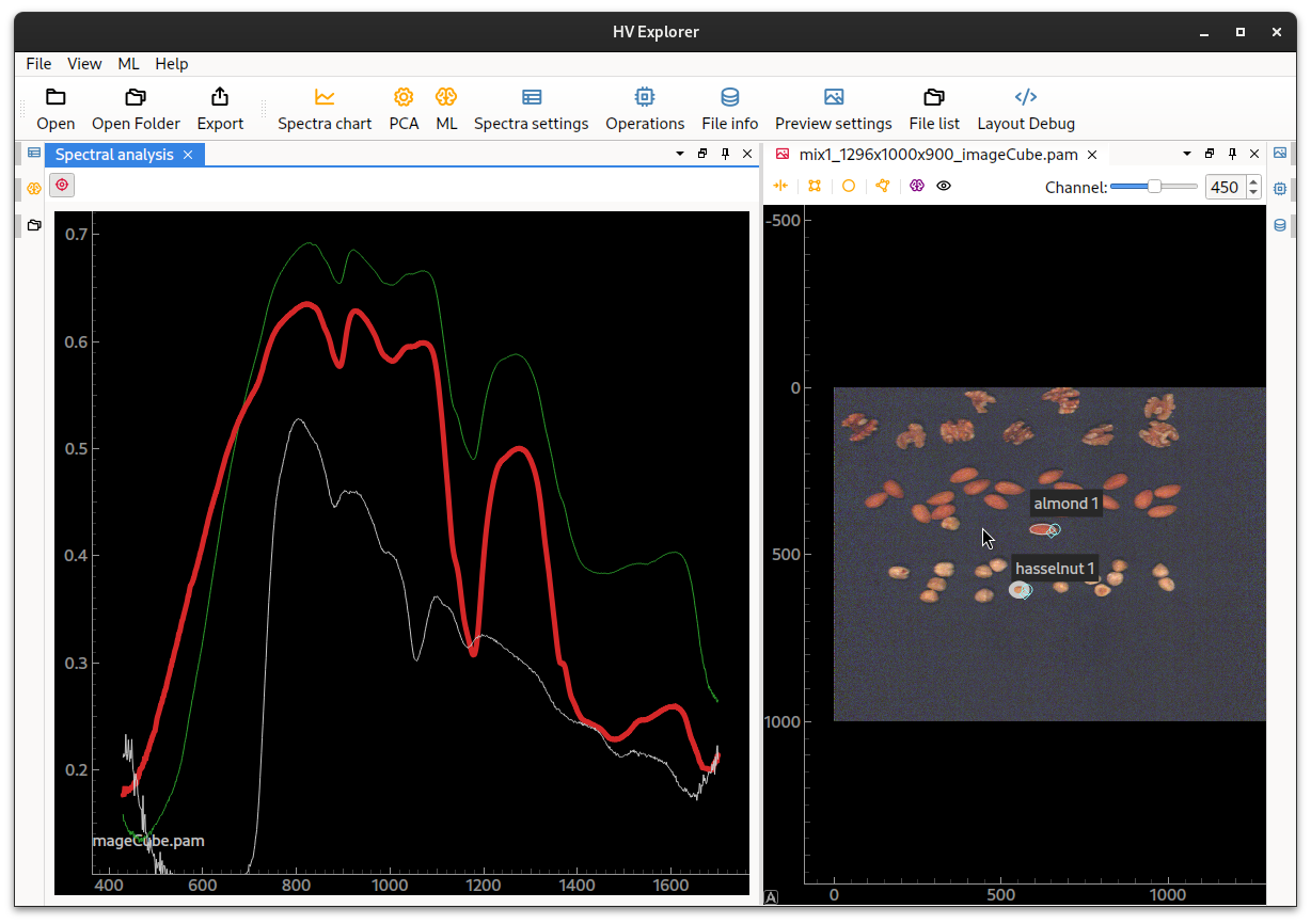
HV Explorer: Spectral chart
Plotting the spectra of the point under the mouse cursor can be toggled by clicking on the "red crosshair" symbol.
Since we have inputed Wavelength information as an operation the plot displays
the wavelengths (in nm) in the Y-axis, otherwise the band/channel number would
be displayed.
Demo
HV Explorer: Spectra chart
Spectra settings
The Spectral analysis panel contains several options that can modify the plots.
HV Explorer: Spectral settings interface
| Number | Name | Description |
|---|---|---|
| 1 | Add property | Create a new property (label or value) Create classes for ML training, PCA visualiztion, ... Properties will appear as new columns alongside "Name" and "Color" |
| 2 | Remove property | Remove a property |
| 3 | Remove spectrum | Remove selected spectrum/ROI |
| 4 | Export spectra data | Export spectra data as CSV, XLSX or JSON |
| 5 | Save annotations | Save ROIs to JSON file Allows using ROIs in python script with HV SDK |
| 6 | Load annotations | Load ROIs from JSON file |
| 7 | Show/hide spectra | Toggle the visualization of the selected spectra on the graph |
| 8 | Spectrum name | Name of the spectrum Double click to edit |
| 9 | Spectrum color | Color of the spectrum Double click to change with a color picker |
| 10 | Filter type | Smooth the spectra The available filters are Gaussian or Savitzky Golay |
| 11 | Enable/disable SNV | Perform normalization of the spectra to facilitate the comparison of different spectra |
| 12 | Enable/disable Continuum removal | Normalize reflectance spectra in order to compare individual absorption features from a common baseline |
| 13 | Show/hide Standart Deviation | Standart deviation of the spectra inside the ROI |
| 14 | Derivative | First or second order derivatives can be shown instead of the pure spectra Useful for comparing different spectra |
Comparing spectra
Now we add more selection areas in order to try and compare the spectra of the different nuts.
Note that even though SNV is enabled is not very easy to spot the differences between the spectra as their general shape is quite similar. With the buggest differences being in the area around 1150nm and 1400nm.
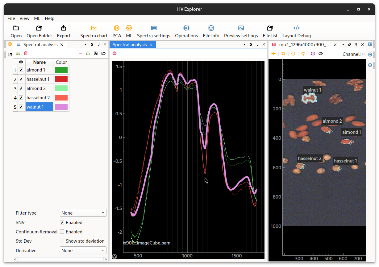
HV Explorer: spectra of almonds, walnuts and hasselnuts
Right click the plot area and select "Plot options->Grid" to enable/disable the X or Y grids in the plot.
These differences can be visualized easier if we use the 1st derivative. There are big difference around 1150nm, 1200nm and 1350nm.
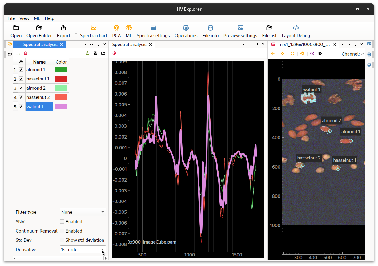
HV Explorer: spectra of almonds versus walnuts (1st derivative)
Demo
HV Explorer: Spectra settings
Datacube slice view
It is also possible to show a slice of the datacube so that all the wavelengths/bands/channels of a single image line are shown as a grey scale image. This corresponds to the original image captured by the camera which has been "stacked" in order to generate the datacube from the scanned lines.
This is done by clicking on the slice icon on the top of the image.
A line, which can be dragged left/right will be shown, demonstrating where the
slice is being made.
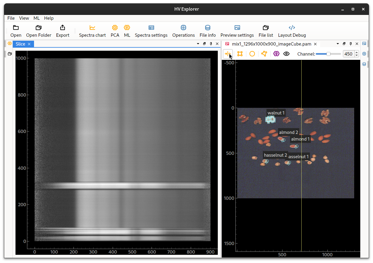
HV Explorer: datacube slice view
Exporting datacubes
Datacubes can be exported by clicking on the Export icon on the top toolbar.
This is useful for for example converting between datacube file formats
(PAM, TIFF and ENVI
currently supported) or changing the interleave type.
It can also be used to export a processed datacube (which has, for example, been
calibrated for reflectance, cropped or had other operations performed on it).
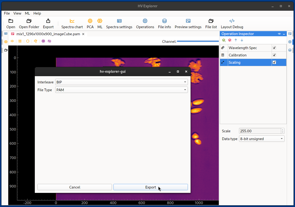
After clicking on Export, the desired interleave type
must be selected (BIL, BSQ or BIP)
as well as the file type (PAM, TIFF or
HDR (ENVI)).
Then a file name must be specified, along with the desired save location.
Note that HV SDK supports all three types of interleave for the three supported file formats, however external applications might expect a specific interleave type depending on the file extension. Therefore, when exporting, it is quite important to choose a proper interleave type for the desired file type: ENVI supports all 3 types of interleave while TIFF is natively BSQ and PAM is natively BIP.
A final consideration before exporting a datacube is the current Data type
(which can be inspected using the Metadata Inspector).
As described in the Reflectance calibration section
the data type of the cube might have been transformed by the Operations applied
to it (for example the Reflectance calibration generates 32-bit floating point
data in the [0-1] range) and some of the file formats support only specific data
types.
PAM, for example, only supports either 8 or 16-bit integer data.
The Data type can be modified using a Scaling operation.
Just selected the desired datatype, in this case 8 or 16-bit unsigned, and then
adjust the Scale to an appropriate value (255 for 8-bit and 65535 for 16-bit).
Besides file format support, changing the Data type is also highly revelant when
considering storage efficiency versus loss of detail in the data: a 32-bit float
contains pottentially 4x more detailed data but takes 4x the storage space (which
might already be quite high for 1Gb datacubes containing 8-bit data).
HV Explorer: exporting datacubes
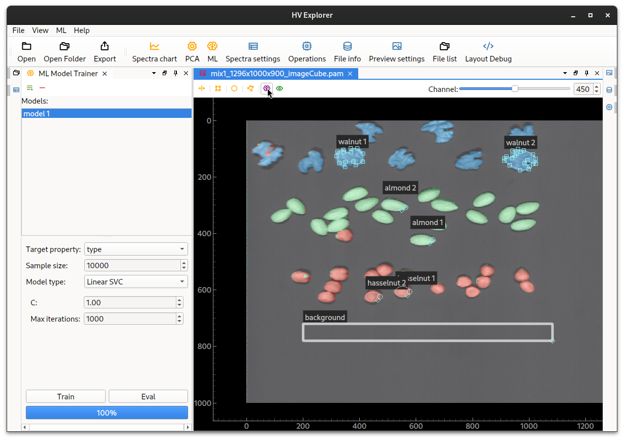
ML models
The HV explorer also supports training ML models for classification.
Start by creating ROIs, at least one for each class that should be indentified. If there is more than one ROI per class it is necessary to group the ROIs under a label property (which can be created under Spectra settings). Create names and assign colors for the labels, then assign the labels to the ROIs.
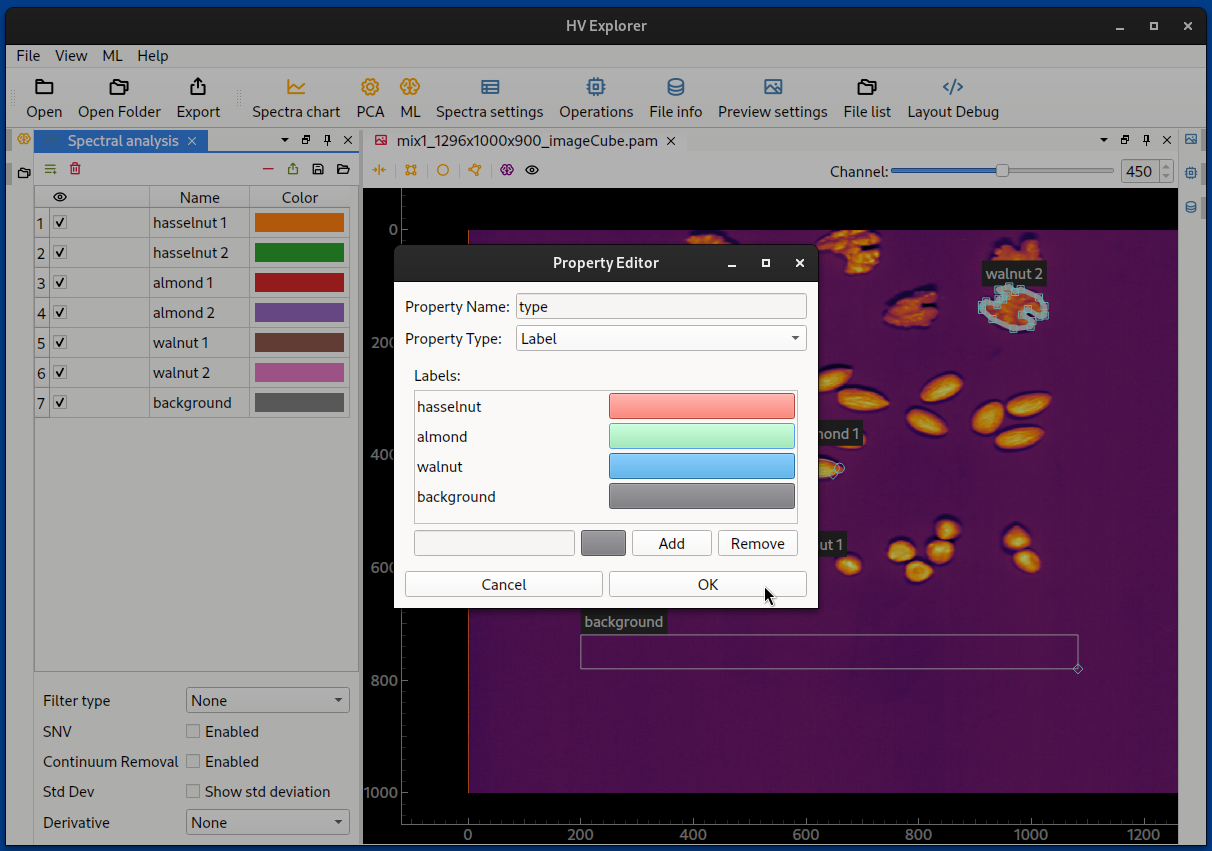
HV Explorer: Add property
HV Explorer: ROIs with properties
It is also possible to use ROIs from multiple images.
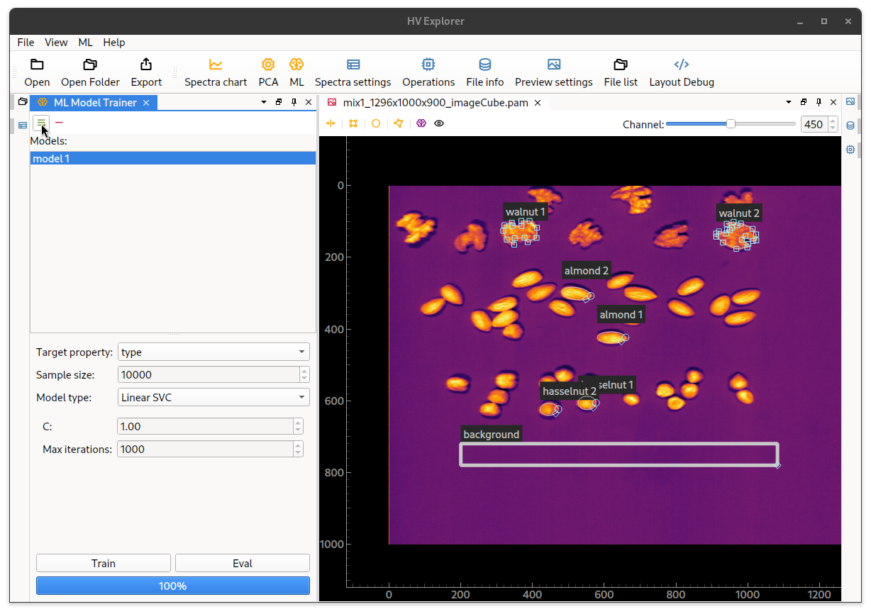
Now open the ML interface (6) and add a model (by clicking on the green icon
on the top).
Select the Target property as the label property created above, or use None
if there is only one ROI per class.
Adjust sample size and model type as desired, as well as the specific model
related parameters.
Then click on Train and wait for the progress bar to show 100%.
The currently supported ML model types are:
- Linear SVC
- SVR
- Least squares
- Regularized least squares
- KMeans
- PLS-DA
HV Explorer: ML interface
Now the result of the model can be overlayed on the image. Click on the "purple brain" icon on the top bar of the image and select the newly generated model. The image will turn gray and after a short while the overlay will be displayed on the image (using the same colors as the input classes).
Enable/disable the overlay by clicking on the "eye" icon (on the top bar of the image).
HV Explorer: ML overlay
It is also possible to apply the ML model as an operation on the datacube.
Start by disabling the ML overlay, then add a new operation of the type
"ML->Apply ML model" in the Operation Inspector.
Choose the newly generated model under the options and click Apply model.
An RGB image containing the classification result will be generated.
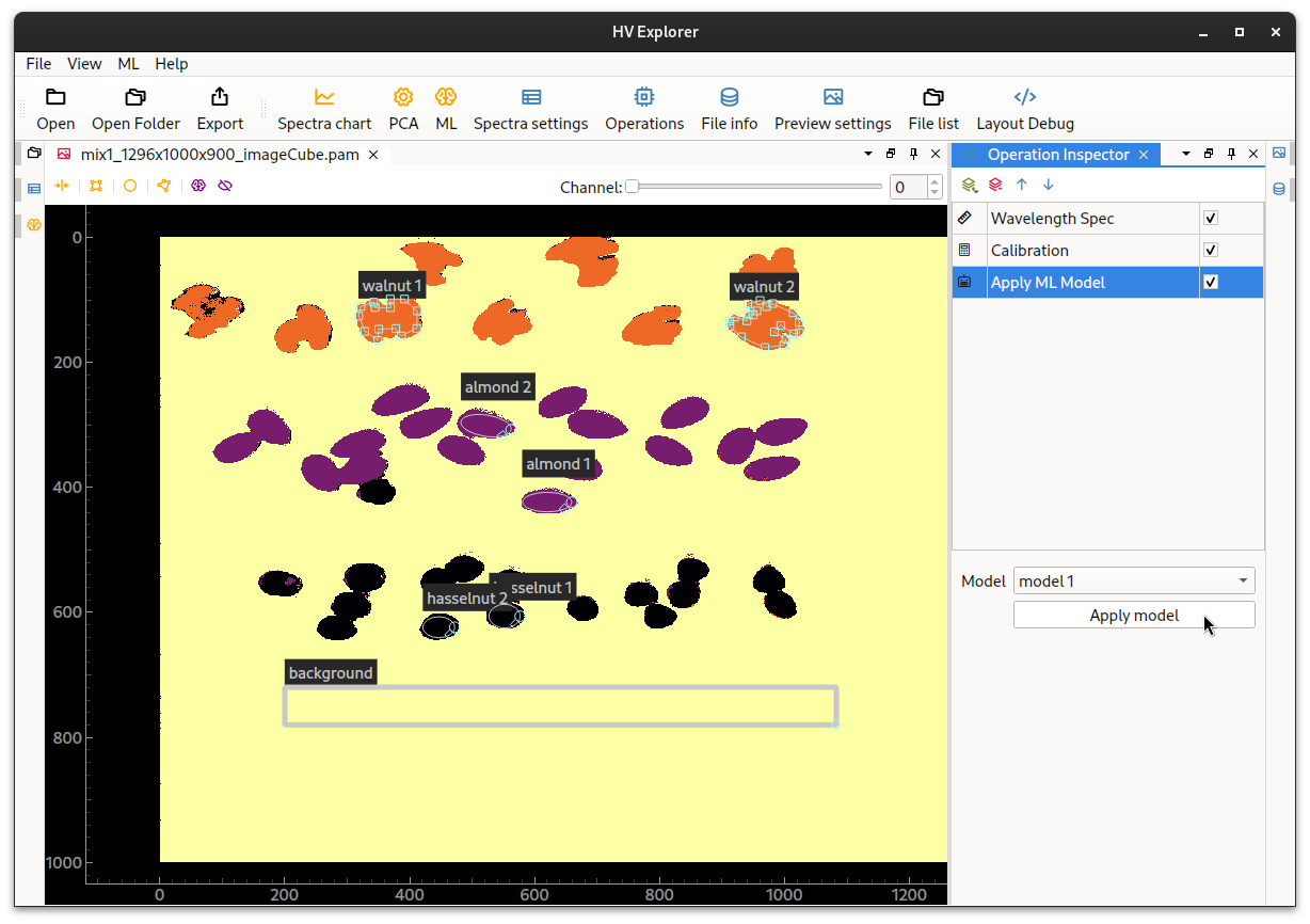
HV Explorer: ML overlay
By using the "Apply ML model" it is possible to generate a model from one or more datacubes and then test the result on another datacube.
Demo
HV Explorer: ML models
PCA view
Open the PCA Viewer by clicking on the PCA (5) button on the top bar.
A PCA will be run on the datacube and sample points of the ROIs will be displayed using the ROI colors (from the Spectra settings panel). This tool is useful for evaluating the separation of the data based on the ROI content. The point under the mouse cursor is plottet as a blue cross.
The PCA component for each axis can be chosen by adjusting the selector on the top PCA bar. If data properties (from the Spectra settings panel) have been created it is possible to select them in the drop down menu to the right, so that their colors are used instead of the ROI colors.
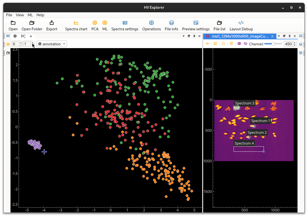
HV Explorer: PCA view
In this example it can be seen that the diffent ROIs don't present enough separation. The background is quite distinct, but the walnuts and hasselnuts are unfortunately quite mixed. And the separation doesn't get much better by changing the PCA components used.
One method that can improve the separation is applying SNV from the
Operations (8) panel in order to normalize the data.
And indeed we can see below that the separation is improved, specially when
inspecting higher PCA components.
This indicates that PCA could be a suitable classification method for this data.
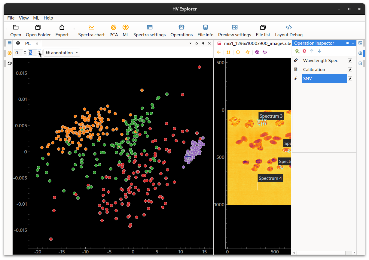
HV Explorer: PCA view with SNV
Demo
HV Explorer: PCA view
PCA operation
For this example we will use the bruised apples example data: cube_reflectance_0_min.pam. For this dataset some apples were dropped and then scanned in order to detect the brown spots hidden under the apple skin. This dataset has already been reflectance calibrated and the spectral channels have been compressed from 900 down to 300 (covering the range from 430 to 1700 nm).
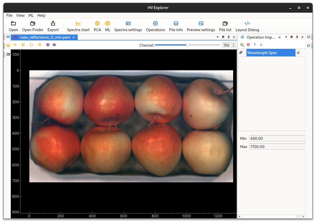
HV Explorer: Bruised apples with false RGB
Note how the bruised stops are almost invisible to the eye on the false RGB image. But by appliying a PCA operation to the datacube the bruises because easily indentifiable in the PCA component number 5. Other PCA components show for example separtion between the apples and the background, as well as other features (see the PCA chapter under the HSI introduction).
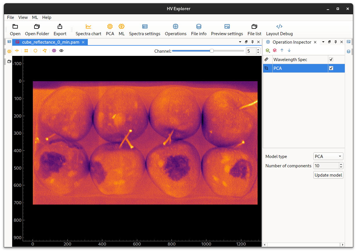
HV Explorer: Bruised apples with PCA
Demo
HV Explorer: PCA operation
Binning
Binning basically means summing a certain amount of pixels together.
Applying a binning operation can be useful for several reasons. It can, for example, help with reducing noise in situations where the input datacube is too dark (scanning of dark objects, limitations in terms of exposure time because of desired high framerate, etc). Another reason to use binning is to reduce the amount of data in order to speed up the training of ML models. Note that in the case of model training, binning should be applied to both the cube used for training as well as the cube where the model should be applied to.
Binning can be applied to the 3 different cube axis (bands, lines and samples)
separately and the amount of pixels to be summed is controlled by the Bin Size
parameter.
Depending on the situation (which axis require higher or lower resolution) it
can be better to apply binning to just some specific cube axis or to all of them.
- lines: number of raw images, corresponding to "image height"
- samples: spatial width
- bands: number of channels/wavelengths
Note that binning in the spacial direction (lines or samples) will alter the aspect ratio of the image. And in that case the ROIs need to be modifed to fit the "new image".
HV Explorer: Binning operation
Since binning is basically a sum it is necessary to check that the data type of the cube is suitable. For example a 8-bit integer is not recommended since it will have a high risk of saturating and clamping. A 16 or 32-bit integer or float type is recommended instead.
The data type can be verified in the File Info (Metadata Inspector).
Modify the data type before applying binning by using either a Scaling
or DType change operation, depending if scaling is also necessary or just the
type change itself.
And if desired, apply scaling after the binning in order to "normalize" the new cube.
Band Selection
The general limiting factor for scaning speeds using the Hypersvision cameras is the system framerate (which is directly proportional to the amount of bands selected). For example, the maximum framerate for the Hypervison1700, with all 900 bands, is 153fps. If a higher scanning speed (belt speed) is desired it is necessary to reduce the amount of selected bands.
It is possible to simulate a scan with a reduced amount of bands by using the
Band selection operation.
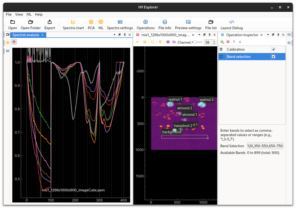
HV Explorer: Band selection operation
Increasing the camera framerate will reduce the maximum possible exposure time, which can cause the image to become darker if there is not enough light available. In this case the Binning operation can be used in order to reduce noise.
Support
Report bugs by writing an email to: hv-explorer-support