Usage Guide
This guide covers the key functions and concepts needed to work effectively with the HV SDK: loading and manipulating hyperspectral datacubes, building lazy processing pipelines, calibrating raw captures to reflectance, and streaming data from a live or simulated camera.
This guide targets the HV SDK v1 Python API.
If you are migrating code written for the pre-1.0 hsi package, see the
v1 migration guide.
Related resources
For a complete API reference, as well as guides on how to work with the framework, see the official documentation.
Refer to the Getting Started and Guide, as well as Recipes, for a complete overview of the HV SDK's capabilities.
Tutorials and Examples
Also check the HV SDK Tutorials and Examples section for runnable examples using the HV SDK.
Most examples also have standalone Python scripts that can be downloaded and
run without editing paths.
Set HSI_EXAMPLE_BASE_DIR to the folder containing the example datacubes,
then use the optional environment variables documented in
Running Downloaded Scripts
to override cubes, annotations, model paths, and output files.
Foundational Concepts
This section covers two concepts that shape how you read, process, and export data with the SDK: how data is laid out in memory (interleave), and when that data actually gets loaded (lazy evaluation). Understanding both up front makes the rest of this guide — and the SDK's behavior in general — more predictable.
Interleave Optimization
Hyperspectral images are inherently three-dimensional, structured by lines (height), samples (width), and bands (spectral channels). The way this 3D data is stored in memory or on disk is known as its interleave type. See Data ordering for the full axis explanation.
Interleave is normally something you have to actively account for to read and process multi-dimensional data correctly and efficiently. The HV SDK tries to make this easier: for most pipeline operations, it handles interleave differences transparently, so correctness doesn't depend on knowing the underlying interleave type.
This section mainly matters in two cases: when you want to optimize the
performance of a processing pipeline, or when you export data to NumPy directly
with to_numpy(), whose axis order depends on the Image's native interleave.
The latter can be sidestepped entirely by using to_numpy_with_interleave()
instead, which lets you specify the layout explicitly.
The HV SDK supports three primary interleave types: BIP (Band-Interleaved-by-Pixel), BIL (Band-Interleaved-by-Line), and BSQ (Band-Sequential).
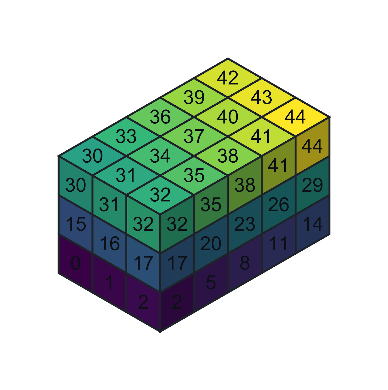
BSQ data ordering
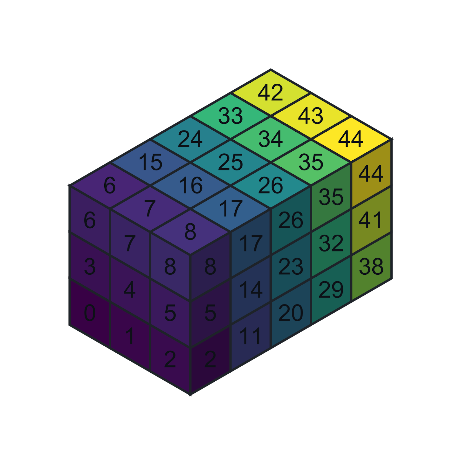
BIL data ordering
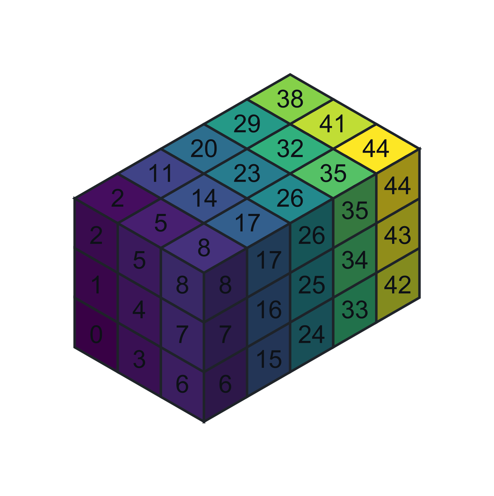
BIP data ordering
Understanding and strategically choosing the interleave type can be crucial for optimizing the performance of your hyperspectral processing workflows. This is because modern CPUs and memory systems operate most efficiently when accessing data that is stored contiguously in memory (cache locality). If an operation frequently accesses data along a specific dimension, aligning the data's interleave with that access pattern can significantly improve processing speed by maximizing cache hits and minimizing memory fetches.
Here's a breakdown of common interleave types and the operations they typically optimize:
| Interleave | Layout | Typically best for |
|---|---|---|
| BIP | L x S x B | Pixel-wise spectral workflows (classification, unmixing) |
| BIL | L x B x S | Line-wise processing across width and/or bands |
| BSQ | B x L x S | Per-band 2D image operations |
-
Performance: Accessing data contiguously (e.g., all elements of a row in a C-contiguous array) is significantly faster due to CPU caching. If your algorithm iterates over bands for each pixel, BIP is generally more efficient. If it processes entire bands as 2D images, BSQ is usually better.
-
Memory Access Patterns: When working with NumPy arrays derived from
Image, understanding the interleave helps you choose the correct axis order for array indexing (arr[lines, samples, bands]vs.arr[bands, lines, samples]), avoiding performance penalties from non-contiguous memory access and preventing logical errors. -
SDK Capabilities: The HV SDK can transform interleave efficiently when needed, but it is still beneficial to align your chosen interleave with your primary operations.
Image.to_interleave()andimg.to_numpy_with_interleave()let you control this explicitly.
By being mindful of interleave type, you can write more efficient and correct hyperspectral data processing code.
BIP (Band-Interleaved-by-Pixel)
- Memory Layout:
[lines, samples, bands](L x S x B) - Optimized for: Operations that require accessing all bands for a single pixel or all bands for a specific spatial location sequentially. This means spectral information for a pixel is stored contiguously.
- Examples: Pixel-wise spectral classification, spectral unmixing, analyzing or comparing individual spectral curves, point-based spectral feature extraction.
- SDK Slicing:
Imageslicingimg[line, sample, :]is inherently optimized for BIP-like access.
BIL (Band-Interleaved-by-Line)
- Memory Layout:
[lines, bands, samples](L x B x S) - Optimized for: Operations that process all samples for a single band within a line or all bands for an entire line sequentially. This means a full line of spectral data is stored together.
- Examples: Line-based spatial filtering applied independently to each band, transformations that operate across the spatial width of a line for all bands, and processing where line-wise access across multiple bands is primary.
BSQ (Band-Sequential)
- Memory Layout:
[bands, lines, samples](B x L x S) - Optimized for: Operations that process an entire 2D image for a single band at a time. This means all spatial data for one spectral band is stored contiguously.
- Examples: Image processing techniques applied to individual bands (e.g., image segmentation, object detection on a specific spectral band), creating grayscale visualizations for individual bands, and band-ratio calculations across the entire image.
Lazy loading
Hyperspectral datacubes are inherently large: their three-dimensional shape
(lines × samples × bands) can reach a gigabyte or more per file, and this gets
worse once data is converted to a wider dtype such as float32 for
calibration or arithmetic. The SDK mitigates this by making pipeline
operations lazy.
The SDK builds a lazy processing pipeline: calling methods on an Image
(slicing, dtype conversion, calibration, reductions, etc.) doesn't immediately
read or compute anything. Each call just returns a new Image describing the
pipeline built so far. Data is only loaded — and only the part of the datacube
actually needed — once the pipeline is triggered.
img = hs.open("path/to/file.hdr")

# Nothing is loaded yet — this only extends the pipeline description
scaled = img.ensure_dtype(hs.float32) / 255.0

# Triggers the load: data is now read from disk and processed
array = scaled.to_numpy()
This keeps RAM usage low, since datacubes are often multi-gigabyte. It also means the cost of a pipeline is paid at the trigger point, not when it's built — if you trigger the same lazy chain more than once, that work (or a camera capture) can be repeated unless you cache the result explicitly.
Common triggers:
- Converting to a NumPy array (
Image.to_numpy()orImage.to_numpy_with_interleave()). - Forcing a cache with
Image.resolve()— see Forcing cache for when to do this explicitly. - In camera pipelines, capture only starts once the pipeline is consumed — see Camera interface.
Basics
This section covers basic functions for reading, writing, and accessing data. It also introduces core data handling patterns used throughout this guide.
Reading and writing datacubes
The SDK supports reading and writing PAM, ENVI and TIFF formats. The format is determined by the file extension.
import qtec_hv_sdk as hs

# Opens an ENVI file
# Data is not yet loaded into memory due to lazy loading
# The data will only be loaded when accessed (e.g., for processing or conversion)
img = hs.open("path/to/file.hdr")

# Writes PAM format
# Data is read from the source as it is written to the file.
hs.write(img, "path/to/output.pam")
Interacting with NumPy
Data can be easily moved between the SDK and NumPy. Note that exporting to NumPy triggers a memory load for the necessary data.
import qtec_hv_sdk as hs

# All 3 methods below cause the necessary data to be read into memory

# Get the full 3D cube
array = img.to_numpy()

# Get the full 3D cube, with the desired memory layout
array = img.to_numpy_with_interleave(hs.bil)

# Get a 2D grayscale image corresponding to a single wavelength band (index 200).
slice_2d = img.array_plane(200, hs.bands)

# Create Image from numpy array
img = hs.Image.from_numpy(array, hs.bsq)
The axis order of the resulting ndarray depends on the native interleave of
the Image. See the Slicing section for details on how this
interacts with indexing, and use to_numpy_with_interleave() for predictable
axis ordering.
Note that explicitly converting the interleave incurs a reordering cost, but
may actually improve downstream performance if your subsequent operations are
better suited to the target interleave — see Interleave Optimization
for guidance on choosing the right layout for your workload.
Data access
Slicing
Use Image.slice() or [] to operate on a specified subset of data.
Note: Slicing indices are always in BIP format: [lines, samples, bands].
# Note that the ordering is always BIP: lines, samples, bands
img[:, :, :]     # The full image
img[:20, :20, :] # The first 20 lines and samples
img[:, :, ::4]   # Take only every 4th band
Slice indices are always in BIP format [lines, samples, bands], regardless
of the image's native interleave. However, to_numpy() returns an array whose
axis order does reflect the native interleave — this mismatch is a common
source of bugs.
To avoid this, prefer to_numpy_with_interleave(hs.bip) for consistent
indexing. If you use to_numpy(), you must check img.meta.interleave
and index accordingly. Explicitly converting the interleave via
to_numpy_with_interleave() incurs a reordering cost, but can be a net
gain if your subsequent operations align well with the target layout. See
Interleave Optimization for guidance.
arr = img.to_numpy()

# the index order depends on the original interleave type
if img.meta.interleave == hs.Interleave.BIL:
    px = arr[line, band, sample] # (Lines, Bands, Samples)
elif img.meta.interleave == hs.Interleave.BSQ:
    px = arr[band, line, sample] # (Bands, Lines, Samples)
elif img.meta.interleave == hs.Interleave.BIP:
    px = arr[line, sample, band] # (Lines, Samples, Bands)
Changing the interleave type
The SDK provides two ways to work with a specific interleave: converting the
Image itself, or specifying the layout only at the point of NumPy export.
-
to_interleave()— converts theImageto a new interleave in the SDK pipeline. Use this when subsequent SDK operations will benefit from a specific memory layout (see Interleave Optimization), or when writing to disk in a particular format (see exporting datacubes). -
to_numpy_with_interleave()— exports to NumPy with a specified axis order without modifying the underlyingImage. Use this when you only need a consistent layout for NumPy indexing and don't need the SDK pipeline to reflect the change.
import qtec_hv_sdk as hs

img = hs.open("path/to/file.hdr")

# Convert the Image itself to BIL — subsequent SDK operations will use this layout
new_img = img.to_interleave(hs.Interleave.BIL)

# Export to NumPy with a specific layout, without changing the Image
arr = img.to_numpy_with_interleave(hs.bil)
Type conversion
The SDK operations preserve the input dtype — conversions are never applied implicitly. This means you should convert before operations that require a specific type, such as division in reflectance calibration (which requires a float type to avoid integer truncation).
Use ensure_dtype() to convert to a target type, or no-op if already correct.
# Raw captures are typically uint8 or uint16.
# Dividing without conversion causes integer truncation — most values become 0.
img = hs.open("image.pam")                         # dtype: uint8
wrong = img / 255                                    # still uint8 — all values 0 or 1

# ensure_dtype() converts only if needed — safe to use even if type is uncertain
correct = img.ensure_dtype(hs.float32) / 255.0     # dtype: float32, values in [0, 1]
as_dtype() is also available and behaves identically, except it always
converts even if the type already matches.
Forcing cache
By default, all SDK operations are lazy — nothing is computed until data is
actually needed. Image.resolve() explicitly triggers computation and stores
the result in memory, returning a new cached Image.
This is useful for intermediate results that are expensive to compute and
reused multiple times in a pipeline. Without resolve(), such results would
be recomputed from scratch each time they are accessed.
The example below shows a manual reflectance calibration pipeline to
illustrate why caching matters. White and dark references are reduced once and
cached with resolve(), then reused in the calibration expression.
For production usage, prefer the SDK's built-in calibration helpers in the
Reflectance calibration section
(make_reference() and reflectance_calibration()), which are clearer and
less error-prone.
import qtec_hv_sdk as hs

img = hs.open("image.pam")
white_img = hs.open("white_ref.pam")
dark_img = hs.open("dark_ref.pam")

# Without resolve(), these reductions would be recomputed every time
# the references are used.
white_ref = white_img.ensure_dtype(hs.float32).mean_axis(hs.lines).resolve()
dark_ref = dark_img.ensure_dtype(hs.float32).mean_axis(hs.lines).resolve()

img = img.ensure_dtype(hs.float32)
calibrated = (img - dark_ref) / (white_ref - dark_ref)
hs.write(calibrated, "calibrated.pam")
Reflectance calibration
Raw hyperspectral data contains sensor-specific artifacts that make direct comparison between pixels or datasets unreliable. Reflectance calibration corrects for these by normalizing against a white reference (a uniformly reflective surface) and a dark reference (captured with the lens covered), converting raw intensity values into physically meaningful reflectance values in the range [0, 1].
The SDK provides make_reference() and reflectance_calibration() in
hs.preprocessing to streamline this process.
import qtec_hv_sdk as hs
from qtec_hv_sdk.preprocessing import make_reference, reflectance_calibration

img = hs.open("path/to/file.hdr")
dark = hs.open("path/to/dark_file.hdr")

# inline white reference
white_ref = make_reference(img[:100, :, :])
dark_ref = make_reference(dark)

reflectance = reflectance_calibration(img, white_ref, dark_ref)

# Note that the data is now of float 32 type
# Consider scaling and converting to 'uint8' to save memory
reflectance_uint8 = (255*reflectance).ensure_dtype(hs.uint8)
make_reference() calls resolve() internally. This forces the reference to be
computed once and cached in memory, so the same white or dark reference can be
reused in multiple calibration pipelines without being recalculated each time it
is used.
Operations
Elementwise operations
The standard arithmetic operators (+, -, *, /) work directly on
Image objects and are applied lazily across the datacube. These are
the building blocks for operations like reflectance calibration and band
arithmetic.
Scalar operations preserve the input dtype. Use ensure_dtype() before
division to avoid integer truncation — see Type Conversion.
# Subtract two bands to highlight spectral differences
diff = img[:, :, 500] - img[:, :, 810]

# Scale image to (0, 1) — convert to float first to avoid truncation
scaled = img.ensure_dtype(hs.float32) / 254.
Reduction operations
Reductions collapse the datacube along a single axis, returning an Image
with that dimension removed. Supported operations are mean, standard deviation,
variance, and sum.
# Collapse the bands axis → 2D spatial image (mean across spectrum)
img.mean_axis(hs.bands)

# Collapse lines then samples → 1D mean spectrum
img.mean_axis(hs.lines).mean_axis(hs.samples)
Matrix multiplication
The dot() method applies a vector or matrix projection along a specified
axis. This is useful for spectral weighting, dimensionality reduction, and
applying learned spectral transforms.
-
A 1D vector operand of shape
(bands,)produces a single-band output — equivalent to a weighted sum across the spectrum per pixel. -
A 2D matrix operand of shape
(n, bands)produces ann-band output, where each output band is one row of the matrix dotted with the spectrum.
# 1D case: weighted sum of bands 2 and 200
operand = np.zeros(920)
operand[2] = 0.5
operand[200] = 0.5
res = img.dot(operand, hs.bands)

# 2D case: two-band output
# Band 0: weighted sum of bands 2 and 200 (same as above)
# Band 1: passthrough of band 25
operand = np.zeros((2, 920))
operand[0, 2] = 0.5
operand[0, 200] = 0.5
operand[1, 25] = 1.0
res = img.dot(operand, hs.bands)
Other operations
The SDK provides several additional pointwise and reduction utilities:
-
binning(n, axis)— averages everynelements along the given axis. Note that the output dtype is not automatically promoted, so useensure_dtype()beforehand if overflow is a risk. -
clip(min, max)— clamps all values to the provided range, useful for removing sensor artifacts or outliers before further processing. -
nan_to_num(value)— replacesNaNvalues with a scalar, typically needed after reflectance calibration where division by zero can occur.
# Apply mean-binning (beware that the dtype will not be changed automatically)
# Use `ensure_dtype()` first if the input type is not big enough to hold the binning results
condensed = img.ensure_dtype(hs.float32).binning(8, hs.bands)

# Clip image to the provided range
clipped = img.clip(0, 1)

# Convert NaN values to the provided value
non_nan = img.nan_to_num(0)
Custom operations
The SDK provides facilities for injecting custom code directly into the lazy pipeline, meaning your functions benefit from the same streaming and lazy evaluation as built-in operations — without loading the full cube into memory.
Use this when the built-in operations do not cover your use case. The most common helpers are:
Image.ufunc()for applying a NumPy function to each frame or plane in the pipeline.- Example: Absorbance Calibration
uses
ufunc()to convert reflectance to absorbance.
- Example: Absorbance Calibration
uses
@hs.util.operationfor defining a custom lazy SDK operation, including access to frame metadata.- Example: Checking for dropped frames uses
@operationto warn from inside a camera pipeline.
- Example: Checking for dropped frames uses
hs.util.predictor()for wrapping scikit-learn-style model inference.- Examples: Visualize Classification Results
and Predict a Regression Map
use
predictor()for lazy model inference.
- Examples: Visualize Classification Results
and Predict a Regression Map
use
hs.ml.pca_helper()for applying a fitted scikit-learn PCA model lazily to anImage.- Example: Fit PCA and Preview Components
uses
pca_helper()to apply a saved PCA transform.
- Example: Fit PCA and Preview Components
uses
Slicing custom operations
Custom operations are lazy just like built-in SDK operations. If you later request only a band, a crop, or a single pixel from the custom-operation output, the SDK tries to fetch only the corresponding input slice from the parent image. That is correct for pointwise same-shape operations, such as absorbance:
import numpy as np

absorbance = reflectance.ufunc(
    lambda meta, plane: -np.log10(np.clip(plane, 1e-6, 1.0))
)
band = absorbance.array_plane(50, hs.bands)
Some operations need more input than the requested output slice. For example,
SNV needs the full spectrum for each pixel even if you only request one output
band. In those cases, pass slice_transform and accept the requested output
slice as a third callback argument:
import numpy as np
import qtec_hv_sdk as hs
from qtec_hv_sdk.util import operation


@operation(hs.bil, slice_transform=lambda out_slice: (slice(None), out_slice[1]))
def snv_line(meta, line, out_slice):
    # BIL plane order is (bands, samples). The slice transform keeps all input
    # bands available but preserves sample slicing from the output request.
    mean = np.nanmean(line, axis=0, keepdims=True)
    std = np.nanstd(line, axis=0, keepdims=True)
    std = np.where(std < 1e-8, 1.0, std)
    normalised = (line - mean) / std
    return normalised[out_slice[0], :]


snv_img = snv_line(reflectance.to_interleave(hs.bil))
single_band = snv_img.array_plane(20, hs.bands)
The same slice_transform argument is available on Image.ufunc(). Use it
when the callback changes the plane shape, reduces an axis, or computes each
requested output value from a wider input region. The transform receives the
requested 2D output-plane slice and returns the 2D input-plane slice that must be
read from the parent image. Both slices use the selected interleave's plane-axis
order: BSQ is (lines, samples), BIL is (bands, samples), and BIP is
(samples, bands).
Applying fitted models lazily
Use hs.util.predictor() when you have a fitted scikit-learn-style model and
want to apply it to an Image without loading the whole cube first. The model
must expose a predict(X) method where X has shape (n_pixels, n_bands).
The SDK handles the line-by-line image pipeline and produces a new Image
with model outputs.
from qtec_hv_sdk.util import predictor

hs_model = predictor(fitted_model)
prediction = hs_model(reflectance_crop)
prediction_map = prediction.to_numpy_with_interleave(hs.bip)[:, :, 0]
Classifiers often return string labels, but image data must be numeric. Wrap string-label classifiers in a small adapter that maps class names to integer ids before returning predictions:
class NumericLabelClassifier:
    def __init__(self, clf):
        self.clf = clf
        self.classes_ = np.array(clf.classes_)
        self.class_to_id_ = {
            class_name: class_id
            for class_id, class_name in enumerate(self.classes_)
        }

    def predict(self, pixels):
        labels = self.clf.predict(pixels)
        return np.array([self.class_to_id_[label] for label in labels], dtype=np.uint8)
For complete workflows, see the classification, regression, and streaming examples.
Operation-based streamed inference
predictor() is the shortest path when you only need the model output. Use
@operation when the streamed line needs custom Python logic around the model:
for example, cleaning NaN values, returning both class ids and a visual band,
or keeping the output compact for a live workflow.
This pattern keeps the workflow as an SDK Image -> Image pipeline, so the same
operation can be applied to a saved cube, a simulated camera, or a real camera
image. The terminal call that consumes the final image drives the capture once.
import numpy as np
import qtec_hv_sdk as hs
from qtec_hv_sdk.util import operation


def make_line_classifier(classifier, visual_band):
    @operation(hs.bil, slice_transform=lambda out_slice: (slice(None), out_slice[1]))
    def classify_line(meta, line, out_slice):
        # BIL plane order is (bands, samples). The model expects
        # (n_pixels, n_bands), so transpose the line before prediction.
        np.nan_to_num(line, copy=False)
        class_ids = classifier.predict(line.T.astype(np.float32))
        visual = line[visual_band, :].astype(np.float32)
        output = np.stack([class_ids, visual], axis=0)
        return output[out_slice[0], :]

    return classify_line


preprocessed = build_preprocessing_pipeline(camera_or_file_image)
# Use the same preprocessing that was used when fitting the saved model.
classified = make_line_classifier(model, visual_band=164)(preprocessed)

# Materialise the compact two-band result:
#   output[:, 0, :] = class ids
#   output[:, 1, :] = visual band
output = classified.to_numpy_with_interleave(hs.bil)
If you need live display or logging, consume the compact image with a terminal
stream loop and keep side effects there. The classifier remains an SDK
Image -> Image operation, while preview code observes each compact line once:
rows = []
with classified.stream() as stream:
    for meta, line in stream:
        if meta.dropped:
            continue
        rows.append(line.copy())
        preview.append(line[0].astype(int), line[1].astype(np.float32))

output = np.stack(rows, axis=0)
Keep GUI, logging, and other side effects in this terminal loop. Lazy
operations can be evaluated more than once depending on downstream access, so
side effects inside an operation can produce duplicate preview rows. The final
stream reads the compact (lines, 2, samples) output, not the full spectral
cube.
Applying fitted PCA lazily
hs.ml.pca_helper() wraps a fitted scikit-learn PCA-like model so it can be
applied inside an Image pipeline without loading the full cube. The model
must expose components_ and mean_.
from qtec_hv_sdk.ml import pca_helper

hs_pca = pca_helper(fitted_pca)
scores = hs_pca(reflectance_crop)
score_map = scores.to_numpy_with_interleave(hs.bip)
For fitting, saving, visualizing loadings, component images, ROI scatter plots, and applying PCA to another cube, see the PCA examples.
Annotations and ROIs
HV Explorer annotations can be loaded with hs.annotations.open() and used
directly with SDK image selections. Each annotation has a descriptor and
properties such as type, concentration, or another user-defined target.
import qtec_hv_sdk as hs
import qtec_hv_sdk.annotations

ann_file = hs.annotations.open("annotations.json")


def annotation_value(value):
    if value is None or isinstance(value, (str, int, float)):
        return value
    try:
        return value[0]
    except TypeError:
        return value


for annot in ann_file.annotations:
    class_name = annotation_value(annot.properties["type"])
    selected = reflectance.select_mask_from_descriptor(annot.descriptor)
    spectra = selected.to_numpy_with_interleave(hs.bip)[:, 0, :]
The selected spectra are ordinary NumPy training data with shape
(n_pixels, n_bands), suitable for scikit-learn classifiers, regressors, or PCA
models.
See the Annotations and ROIs examples for complete runnable scripts that extract ROI spectra and draw annotations on a preview image.
Do not estimate performance by randomly splitting pixels from the same ROI or physical sample into train and test sets. Neighboring pixels are highly similar, so that split can make models look better than they really are. Prefer held-out ROIs, separate scans, or independent physical samples.
Plotting annotations
The annotation module also includes Matplotlib helpers for drawing ROI descriptors on top of preview images. These helpers are useful for quick notebooks, QA plots, and documentation figures.
import matplotlib.pyplot as plt
import qtec_hv_sdk as hs
import qtec_hv_sdk.annotations

ann_file = hs.annotations.open("annotations.json")

fig, ax, patches = hs.annotations.plot_image_with_annotations(
    preview_rgb,
    ann_file,
    label=True,
    show_axes=False,
)
plt.show()
For more control, draw on an existing axis:
fig, ax = plt.subplots()
hs.annotations.draw_image(ax, preview_rgb)
hs.annotations.draw_annotations_file(ax, ann_file, label=True)
plt.show()
Available helpers include:
descriptor_patch(descriptor, **patch_kwargs)creates a Matplotlib patch for one descriptor.draw_descriptor(ax, descriptor, label=None, **patch_kwargs)draws one descriptor on an existing axis.draw_annotation(ax, annotation, label=False, color=None, **patch_kwargs)draws one annotation.draw_annotations(ax, annotations, label=False, colors=None, **patch_kwargs)draws multiple annotations.draw_annotations_file(ax, file, label=False, color_property=None, **patch_kwargs)draws an annotation file.draw_image(ax, image, show_axes=False, **imshow_kwargs)draws an image withimshow.plot_image_with_annotations(image, annotations, ...)creates or reuses an axis, draws the image and annotations, and returns(fig, ax, patches).
The plotting helpers are currently ahead of the published API reference. The official annotations guide will cover them when it is updated.
Camera interface
The SDK connects directly to a Hypervision camera over Ethernet, providing
control over exposure, framerate, spatial crop, and spectral bands. Once
configured, the camera is represented as an Image, meaning the same lazy
pipeline operations used for file-based data apply equally to live capture.
import qtec_hv_sdk as hs
from datetime import datetime


def current_datetime_filename():
    return datetime.now().strftime("%Y-%m-%d_%H-%M-%S")

N_IMGS = 10
filename = f"/tmp/_HSI_{current_datetime_filename()}"
SAVE_CUBE = True

# Desired settings
EXP = 1000
FPS = 100
# Horizontal crop
H_START = 200
H_END = 300
# Bands
V_START = 0
V_END = 920

# ETH_B interface
cam = hs.control.Camera("10.100.10.100")

# Get information
print(f"{cam.get_config()=}")
print(f"{cam.get_settings()=}")
print(f"{cam.get_crop()=}")
print(f"{cam.get_exposure()=}")
print(f"{cam.get_framerate()=} {cam.get_framerate_list()=}")
#print(f"Binning: {cam.get_horizontal_binning()}x{cam.get_vertical_binning()}")
print(f"{cam.get_bands()=}")
#print(f"{cam.get_wavelengths()=}")

# Set parameters
print(f"{cam.set_exposure(EXP)=}")
print(f"{cam.set_framerate(FPS)=}")
#cam.set_horizontal_binning(1)
#cam.set_vertical_binning(1)
print(f"{cam.set_horizontal_crop(H_START, H_END)=}")
print(f"{cam.set_bands([(V_START, V_END)])=}")
# Multiple band intervals (up to 8 regions):
#print(f"{cam.set_bands([(V_START1, V_END1), (V_START2, V_END2)])=}")

######### Datacube Capture

# Set camera parameters before creating the Image pipeline or starting a
# direct stream, so references, captures, and streamed lines use the intended
# exposure, framerate, crop, and band selection.
img = cam.to_hs_image()

# Compose lazy processing before capture starts
# Add calibration or other processing here
processed = img.ensure_dtype(hs.float32) / 255.0

# Configure the datacube size (N_IMGS)
datacube = processed[:N_IMGS, :, :]

# Write to file or convert to numpy:
# triggers the streaming start
if SAVE_CUBE:
    #hs.write(datacube, filename + ".pam")
    hs.write(datacube, filename + ".hdr")
    #hs.write(datacube, filename + ".tif")
else:
    array = datacube.to_numpy()

# Also triggers the streaming start
#cube = datacube.resolve()
cam.to_hs_image() builds a lazy camera pipeline; it does not start capturing
data by itself. Capture starts when something consumes the pipeline, such as
to_numpy(), resolve(), hs.write(), or iterating over a stream. This lets
you compose calibration, preprocessing, band selection, or model prediction
before any camera data is requested.
Use one terminal operation for each live capture. If you write one lazy branch and resolve another lazy branch from the same camera image, you may trigger two consecutive acquisitions. If you need multiple operations on the same captured cube, resolve once and reuse the resolved image, or write once and reopen the saved file for offline inspection.
The SDK can also run directly on the camera. In that case, use the same SDK
camera interface, but connect to the local camera service with localhost or
127.0.0.1 instead of the external Ethernet address:
cam = hs.control.Camera("127.0.0.1")
This still streams through the camera service over the REST/TCP interface, but the local connection avoids the throughput limits of the external Ethernet interface. If you need direct local V4L2 access today, use qamlib for capture and combine it with SDK processing as needed. See the qamlib capture with SDK processing example. Direct V4L2 access from the SDK is planned for a future release.
See also the more complete example under the Quick Start section, the streaming examples, and be aware of data throughput limitations.
Simulated Camera
The SDK can also simulate the output of a HSI camera by providing an input datacube.
When a file-backed simulated camera is created from a BSQ datacube, the SDK
converts it to a line-first layout for streaming. This is a BSQ-specific
adjustment: the camera abstraction assumes a push-broom source, so the important
part is that lines are the first dimension. BIL and BIP are both already
line-first for this purpose, so they do not need the same conversion. This means
typical saved cubes can be passed directly to hs.control.Camera() without
manually converting them first.
If the saved file already contains wavelength metadata, the simulated camera can
report those wavelengths directly. ENVI files can store wavelength metadata in
the header, but PAM files normally do not, so add SpectralMeta before creating
the simulated camera when the source file does not carry the camera wavelength
axis. This lets simulated-camera examples use wavelength-based band selection in
the same way as real camera code.
import numpy as np
import qtec_hv_sdk as hs

src_img = hs.open("path/to/file.hdr")

# Optional: tag saved cubes with the camera wavelength axis so a simulated
# camera reports meaningful wavelengths.
meta = src_img.meta
meta.spectral = hs.SpectralMeta(
    wavelengths=hs.WavelengthMeta(
        np.linspace(430, 1700, src_img.meta.shape.bands),
        hs.WavelengthUnit.Nanometer,
    )
)
src_img = src_img.with_meta(meta)

cam = hs.control.Camera(src_img)

# The simulated camera now exposes the same wavelength-style metadata that
# real camera code expects.
wavelengths = np.array(cam.get_wavelengths())
band_650 = int(np.argmin(np.abs(wavelengths - 650.0)))
print(f"Closest band to 650 nm: {band_650}, wavelength={wavelengths[band_650]:.1f} nm")

# Create a stream object
img = cam.to_hs_image()

# Configure the datacube size (N_IMGS)
datacube = img[:N_IMGS, :, :]

# Use the wavelength-derived band index in the normal BIP slicing API.
band_image = datacube[:, :, band_650]

# Trigger the streaming start
cube = datacube.resolve()
# array = datacube.to_numpy()
# band_array = band_image.to_numpy()
Streaming individual frames
Available in the v1 camera API.
Use cam.stream() when you want immediate access to each captured frame. Each
frame returned by the stream is already an eager 2D NumPy array, not an
Image. For a push-broom camera or simulated source using BIL interleave,
this frame normally represents one scan line with shape (bands, samples).
By default, cam.stream() runs until you stop it. A simulated camera backed by
a file also behaves like an open-ended camera source and loops the file from the
beginning. Use cam.stream(n_frames=...) when you want a bounded direct frame
stream.
cam.stream() returns a Python iterator, so prefer
for meta, frame in stream: for most loops. Python handles StopIteration
internally, and the loop simply ends when a bounded stream is done. Use
stream.get_frame() only when you need to request frames manually. For a
bounded direct camera stream, get_frame() returns None when the stream is
exhausted.
cam.stream() gives direct access to eager camera frames. If you instead build
a lazy pipeline with cam.to_hs_image() and call .stream() on the processed
Image, the stream yields processed pipeline output. A simulated direct
camera stream backed by a file loops by default, while a processed Image
stream from a finite simulated source stops when the file is exhausted.
The accompanying meta object contains frame metadata such as sequence number,
timestamp, and whether the frame was dropped.
import qtec_hv_sdk as hs

cam = hs.control.Camera("10.100.10.100")

# Context manager usage:
with cam.stream(n_frames=100) as stream:
    for meta, frame in stream:
        if meta.dropped:
            print(f"Dropped frame {meta.seq} at {meta.timestamp}")
            continue

        # frame is a 2D NumPy array, not an Image pipeline object
        print(f"Frame {meta.seq}: shape={frame.shape}")

# Manual usage
stream = cam.stream(n_frames=100) # Start streaming
try:
    while True:
        item = stream.get_frame()
        if item is None:
            break

        meta, frame = item

        if meta.dropped:
            print(f"Dropped frame {meta.seq} at {meta.timestamp}")
            continue

        print(f"Frame {meta.seq}: shape={frame.shape}")
finally:
    stream.stop()
Choosing a camera workflow
Choose the camera pattern from the shape of the task:
-
Capture a finite datacube: use
cam.to_hs_image(), slice the line dimension to the number of lines you want, then callhs.write(),to_numpy(), orresolve(). Use this when you want to save, inspect, or process a bounded cube. -
Inspect lines directly: use
cam.stream()when you need direct frame-by-frame control, for example reading metadata, handling dropped frames, updating a UI, or sending one line at a time to another system. Each frame is an eager NumPy array. -
Stream processed lines: use
cam.to_hs_image()to compose calibration, preprocessing, band selection, or model prediction, then call.stream()on the processedImage. Use this when you want lazy SDK pipeline operations and line-by-line output at the same time.
The processed-stream pattern looks like this:
img = cam.to_hs_image()[:100, :, :]
processed = img.ensure_dtype(hs.float32) / 255.0

with processed.stream() as stream:
    for meta, processed_line in stream:
        ...
See the streaming examples for full camera pipelines with calibration, classifiers, and regressors.
Push-broom cameras stream one line at a time, and BIL is usually the natural
layout for those frames. When calibrating a camera pipeline, make sure the dark
and white references use the same interleave as the camera output before passing
them to reflectance_calibration().
Checking for dropped frames
The direct stream loop above is usually the simplest place to check for dropped
frames. If you are working inside a lazy Image pipeline instead, dropped
frames can also be detected inside an @operation function so warnings
propagate alongside the data.
Use @operation when you need custom per-frame logic inside the SDK pipeline:
logging dropped frames, applying a NumPy transform, or inserting a small custom
step between built-in SDK operations. If you only need built-in operations such
as calibration, dtype conversion, band selection, or hs.util.predictor(), you
can usually compose them directly on cam.to_hs_image() and stream the result
without writing a custom operation.
import qtec_hv_sdk as hs
import numpy as np
import logging
from qtec_hv_sdk.util import operation

logger = logging.getLogger("main")

cam = hs.control.Camera("10.100.10.100")

@operation(hs.bil)  # tells the SDK to deliver frames in BIL layout to match camera output
def op(meta: hs.FrameMeta, frame: np.ndarray) -> np.ndarray:
    if meta.dropped:
        logger.warning(f"Dropped frame {meta.seq} at time {meta.timestamp}")

    # Do some processing here
    # ...

    return frame

out_img = op(cam)

# Any method call that fetches data from the pipeline will now issue warnings
# if a dropped frame is encountered.
first_100_lines = out_img[:100, :, :]
first_100_lines.to_numpy()
Lab Scanner interface
The SDK can also coordinate a push-broom camera with a lab scanner stage,
conveyor belt, and lights. This is exposed through hs.control.StageController
for real scanner hardware and hs.control.SimulatedStageController for replaying
saved cubes while testing the same high-level workflow.
The generic lab scanner interface is intended for current qtec scanner models such as HyperScan. HyperScan was developed with native HV Explorer and HV SDK support in mind, so it is the recommended scanner model for new SDK-controlled lab scanner workflows. In the SDK-controlled HyperScan workflow, camera FPS and belt velocity are linked: set either FPS or velocity, then the controller calculates the other value from distance, oversampling, and scan geometry.
The Buteo was developed by Newtec as a stand-alone lab scanner, where a host-PC controls the screen, camera, lights, and belt. The SDK supports Buteo integration primarily for existing installations, but it requires extra hardware and software setup before it can be controlled through the same HV SDK workflow. For new systems, prefer HyperScan when SDK and HV Explorer integration are required.
See the official stage-controller guide
for more information on the SDK StageController API.
This functionality is still being tested and the interface may therefore change.
The Buteo Lab Scanner from Newtec requires hardware and software setup before the camera can control the stage, belt, and lights directly (instead of having the host-PC controlling them). This includes switching cables inside the cabinet and booting the camera from a suitable software image.
Contact qtec for the correct setup procedure for the scanner model you are using. See qtecOS Image for more information on creating required bootable media when a camera-side software image is needed.
When the camera controls the Buteo belt and lights directly, the scanner's built-in UI is unavailable. Configuration and control should then be done from a Python script using HV SDK, either on an external PC or from the camera terminal.
This process is also easily reversible if it is desired to go back to original host-PC based functionality.
import qtec_hv_sdk as hs
from datetime import datetime


def current_datetime_filename():
    return datetime.now().strftime("%Y-%m-%d_%H-%M-%S")


# Settings
BIT_MODE = 8
WIDTH = 1280
N_BANDS = 920
EXP_TIME = 3000  # max exposure ~10.000 us at 100fps

TARGET_DIR = "/tmp/"
filename = f"_HSI_{current_datetime_filename()}"

# Camera IP
scanner = hs.control.StageController("10.100.10.100")

# FPS and belt velocity are linked by the stage controller. Set one of them;
# the scanner calculates the other from the scan geometry and oversampling.
# We recommend setting the max fps for the available 1 Gbit/s connection.
# The actual throughput seen experimentally for the 1 Gbit/s connection is
# 12-15% lower than the max theoretical value.
MAX_FPS = pow(2, 30) / (WIDTH * N_BANDS * BIT_MODE) * 0.85
# print(f"{MAX_FPS=}")

# Set conveyor belt velocity in mm/s
# scanner.velocity = 20.0

# Max fps for the 1 Gbit/s connection ~100 for 1280px x 900 bands
scanner.set_fps(MAX_FPS)

# Set conveyor move distance in mm.
scanner.distance = 50.0

# Set oversampling (lines). An oversampling of 4x gives a correct aspect ratio
# visually for this scanner/camera setup.
scanner.oversampling = 4.0

# Adjust camera settings
exp_time = scanner.hs_camera.set_exposure(EXP_TIME)

# Gain is not available at the moment so it is fixed at 1x
# gain = scanner.hs_camera.set_gain(0)

# Change crop top in config if required by the scanner model (Buteo only)
config = scanner.hs_camera.get_config()
print(f"{config=}")
# cal = config.calibration
# cal.crop_top = 20  # must be multiples of 4
# config.calibration = cal
# config = scanner.hs_camera.set_config(config)
# print(f"{config=}")

# Adjust spatial cropping
# crop = scanner.hs_camera.get_crop()
# crop = scanner.hs_camera.set_horizontal_crop(0, crop.max_width)
# crop = scanner.hs_camera.set_horizontal_crop(H_START, H_END)
h_crop = scanner.hs_camera.set_horizontal_crop(0, WIDTH)
print(f"{h_crop=}")

# Adjust number of bands or band intervals
# bands = scanner.hs_camera.get_bands()
# Multiple band intervals (up to 8 regions):
# bands = scanner.hs_camera.set_bands([(V_START1, V_END1), (V_START2, V_END2)])
bands = scanner.hs_camera.set_bands([(0, N_BANDS)])
print(f"{bands=}")

# Convert to Image object
image = scanner.to_hs_image()

# Do not change settings after this point.

# Consuming the image starts streaming plus stage/lights. Use one terminal
# operation for a live scanner capture. This example writes the scan to disk.
# The SDK supports PAM, ENVI and TIFF.
hs.write(image, TARGET_DIR + filename + ".hdr")
# hs.write(image, TARGET_DIR + filename + ".pam")
# hs.write(image, TARGET_DIR + filename + ".tiff")

# Save the current settings to a txt file as well if desired
try:
    with open(TARGET_DIR + filename + "_settings.txt", "w") as f:
        f.write("--- Camera Configuration ---\n")
        f.write(f"{filename=}\n")
        f.write(f"{config=}\n")
        f.write(f"{bands=}\n")
        f.write(f"{exp_time=}\n")
        f.write(f"{h_crop=}\n")
        f.write(f"scanner.fps={scanner.get_fps()}\n")
        f.write(f"{scanner.distance=}\n")
        f.write(f"{scanner.oversampling=}\n")
        f.write(f"{scanner.velocity=}\n")
    print(f"Successfully saved settings to {filename}")
except Exception as e:
    print(f"An error occurred: {e}")
The Lab Scanner image follows the same lazy-capture rules as the camera image pipeline described above.
Simulated stage controller
Use hs.control.SimulatedStageController when you want to test the same
StageController-style workflow without lab scanner hardware. It is backed by an
SDK image, exposes the same high-level properties and methods as
StageController, and provides an image-backed hs_camera. Motion and light
commands are accepted as no-ops, so code that calls toggle_lights(),
set_lights_with_timer(), move_direction(), or stop() can still run during
development.
If the saved cube does not already contain wavelength metadata, tag it before creating the simulated controller so the simulated camera reports meaningful wavelengths.
import numpy as np
import qtec_hv_sdk as hs

source = hs.open("saved_lab_scanner_capture.pam")
meta = source.meta
meta.spectral = hs.SpectralMeta(
    wavelengths=hs.WavelengthMeta(
        np.linspace(430, 1700, source.meta.shape.bands),
        hs.WavelengthUnit.Nanometer,
    )
)
source = source.with_meta(meta)

scanner = hs.control.SimulatedStageController(source, fps=30.0, distance=50.0)

# Camera code can now query wavelengths from the simulated scanner camera.
wavelengths = np.array(scanner.hs_camera.get_wavelengths())
band_650 = int(np.argmin(np.abs(wavelengths - 650.0)))
print(f"Closest band to 650 nm: {band_650}, wavelength={wavelengths[band_650]:.1f} nm")

# The same high-level API can be used by code that normally talks to lab scanner
# hardware. Motion and light calls are no-ops in the simulator.
scanner.set_fps(30.0)
scanner.distance = 50.0
scanner.oversampling = 4.0

image = scanner.to_hs_image()

# Consume a bounded image to trigger the simulated scanner workflow once.
captured = image[:10, :, :].resolve()
band_image = captured[:, :, band_650]

print(captured.shape)
print(band_image.shape)
The hs.control.StageController communicates directly with a REST API interface
running on the camera at <camera_ip>:5001.
Information about the available endpoints for controlling scanner motion and
lights is available in the live documentation at <camera_ip>:5001/docs.