Advanced Processing and Export

This page covers workflow steps that reduce noise, data size, or model input complexity before export or downstream analysis. It explains when to use preprocessing, crop, binning, band selection, PCA component images, and how to export processed datacubes safely.

Spectral preprocessing

Spectral preprocessing can reduce variation that is unrelated to the material property of interest. It should be chosen based on the data and analysis goal, not applied automatically.

Method	Typical purpose
SNV	Centers and scales each pixel spectrum to reduce multiplicative intensity and scattering differences.
Smoothing	Reduces high-frequency noise, but can also suppress narrow spectral features.
Derivatives	Emphasize changes in spectral shape and reduce baseline effects, while often amplifying noise.
Continuum removal	Compares absorption features relative to a local spectral continuum.

Viewer settings and workflow operations

Preprocessing in the Spectral Viewer affects only plotted and exported spectra. This is useful for exploration. It does not change the pixels used by PCA, ML models, or datacube export.

To apply SNV to the complete datacube, add an SNV operation in the Workflow editor. Place it after reflectance calibration and before PCA, model training, model application, or export. HV Explorer currently provides more exploratory preprocessing choices in the Spectral Viewer than as full-cube workflow operations.

Reproduce preprocessing

A trained model expects the same preprocessing and operation order used during training. Apply identical calibration, SNV, binning, band selection, and wavelength ordering to new datacubes before prediction.

SNV Demo

HV Explorer: Spectral Viewer

Crop

The Crop operation keeps a rectangular spatial region of the datacube and removes data outside it. Cropping can reduce processing time and file size when only part of the scanned area is relevant.

Add Crop in the Workflow editor, then set the minimum and maximum coordinates for Lines and Samples. The maximum values are exclusive: a line range of 100 to 200 keeps lines 100 through 199.

Setting	Spatial direction
Lines min/max	Image height or scan direction.
Samples min/max	Image width.

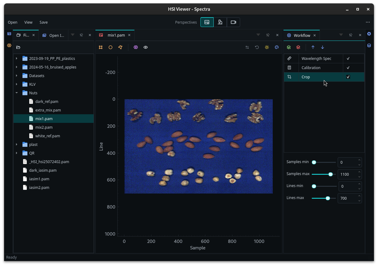
HV Explorer: Crop operation

Annotation coordinates

Cropping changes the spatial origin and image dimensions. HV Explorer automatically adjusts ROIs while the operation is active so that they still cover the same physical sample region. However, saved annotations are tied to the processed cube geometry. Reuse saved annotations only with cubes that have the same crop and operation order, and verify ROI alignment before PCA or model training.

tip

For the smallest intermediate data, place Crop early in the pipeline. Keep calibration before Crop when the white and dark references need the original spatial geometry.

Demo

HV Explorer: Crop operation

Binning

Binning averages neighboring values along a selected datacube axis. It reduces the cube resolution and data volume while often reducing random noise. The operation can be applied independently along Lines, Samples, or Bands using the selected Bin size.

Axis	Effect
Lines	Reduces spatial resolution along the image height or scan direction.
Samples	Reduces spatial resolution across the image width.
Bands	Reduces spectral resolution by averaging neighboring bands.

Binning can be useful when:

• random noise is more important than preserving the finest spatial or spectral detail;
• dark samples or short exposure times produce noisy measurements;
• smaller cubes are needed for faster analysis, model training, or export;
• the intended camera configuration uses lower spatial or spectral resolution.

To apply binning, add a Binning operation in the Workflow editor, choose an axis and bin size, and repeat the operation for any additional axes that should be reduced.

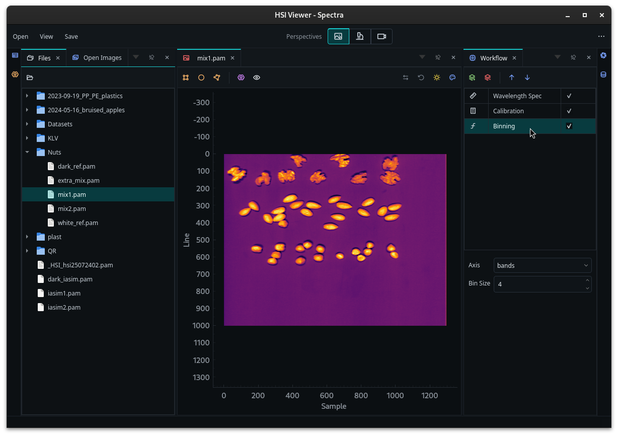
HV Explorer: Binning operation

Spatial coordinates and model inputs

Binning along Lines or Samples changes the image dimensions. HV Explorer automatically adjusts ROIs while spatial binning is active so that they still cover the same physical sample region. However, saved annotations are tied to the processed cube geometry and should only be reused with cubes that have the same spatial binning and operation order.

Binning along Bands changes the model input features and wavelength sampling. Apply the same binning and operation order to training and prediction data when using an ML model.

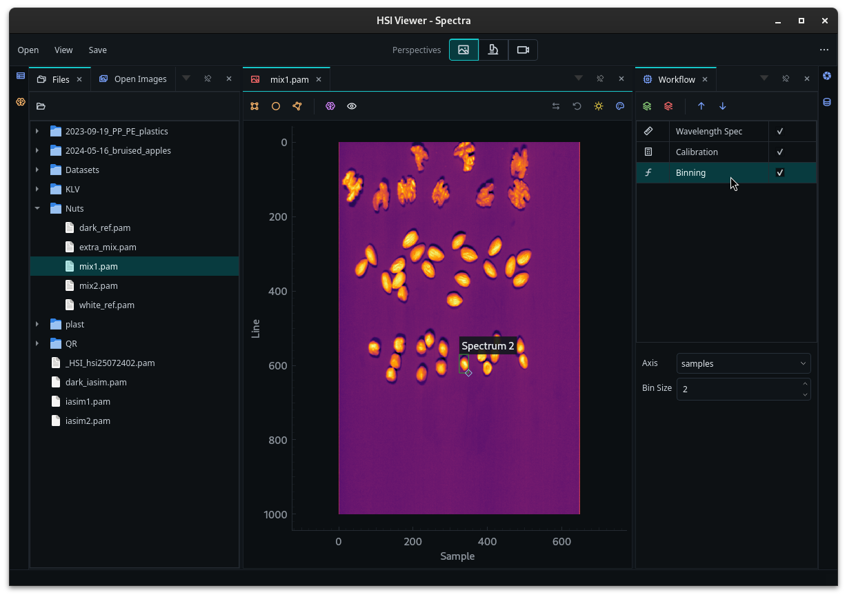
HV Explorer: Binning operation

Data type

HV SDK operations preserve the input data type. Converting integer data to float32 before mean binning avoids loss of precision from integer averaging. Use a DType Change operation before binning when this precision matters, and use Scaling later if an integer output is required for export.

Demo

HV Explorer: Binning operation

Band Selection

Band selection keeps only the spectral channels needed for an analysis or capture workflow. Reducing the number of bands decreases data volume and can speed up processing, model training, and camera acquisition. On a camera, a smaller band selection can support a higher frame rate, although the available exposure time decreases as the frame rate increases.

The Band selection operation can be used on an existing datacube to simulate or prepare a reduced-band workflow:

1. Add Band selection in the Workflow editor.
2. Enter the band indices or index ranges to retain.
3. Apply the operation and inspect the resulting shape and wavelengths in the Metadata inspector (#13).

The operation uses zero-based band indices rather than wavelength values. Enter individual indices separated by commas, or ranges such as 3-5. In the current version, the upper range value is exclusive, so 1,3-5,7 keeps bands 1, 3, 4, and 7. Use the datacube wavelength metadata or Spectral Viewer to identify the indices corresponding to the desired wavelengths.

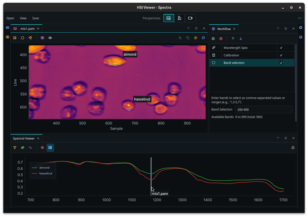
HV Explorer: Band selection operation

Finding relevant bands

For classification workflows, start by looking for wavelength regions where the classes you want to separate have different spectral responses.

• Use the Spectral Viewer to compare ROI spectra from each class. Look for peaks, dips, slopes, or absorption features that differ consistently between classes, then select bands around those wavelengths.
• Try spectral preprocessing in the Spectral Viewer, such as SNV, continuum removal, or first- and second-order derivatives. These views can make differences in shape, baseline, or absorption features easier to identify.
• Use the PCA view to check whether the annotated classes separate. Inspect the PCA loadings and change the displayed loading channels to find wavelength regions that contribute strongly to the separation.

The selected bands should still be checked in the final workflow. A band that looks useful in one sample set may be sensitive to noise, illumination, or sample variation in another.

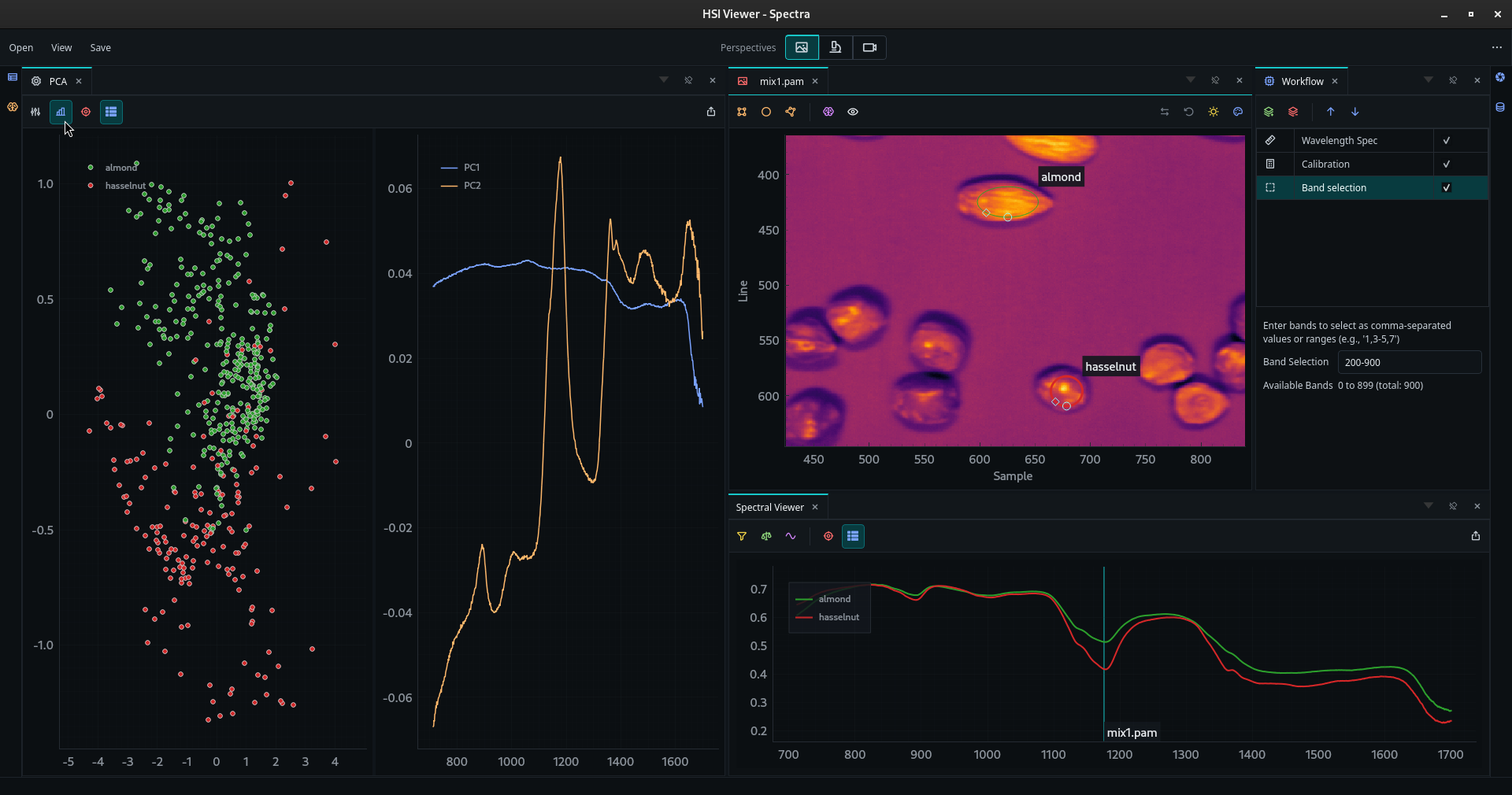
HV Explorer: PCA loadings and spectral plot to find relevant bands

In this example, the Spectral Viewer is used to compare the average spectra for the annotated classes, while the PCA view shows how those classes separate in score space. The PCA loading plot helps identify which wavelengths contribute most to the selected component. Bands near strong class differences in the spectra, or near large positive or negative loading values, are good candidates for a reduced band selection. In the example image, one useful candidate region is around 1180 nm, where the almond and hazelnut spectra differ and the PC2 loading shows a strong feature.

Keep model features consistent

A model must receive the same selected bands in the same order during training and prediction. Record the selected indices and preserve the corresponding wavelength metadata when exporting or reproducing the workflow in the HV SDK.

Balancing speed and signal quality

Higher camera frame rates reduce the maximum available exposure time and may produce darker, noisier captures. Adequate illumination should be considered first; spectral or spatial binning can then trade resolution for lower noise and smaller data volumes where appropriate.

PCA operation

Unlike the ROI-based PCA view, the PCA operation processes the complete datacube and returns a new cube containing PCA component images. These images show spatial patterns associated with the main sources of spectral variation and can be inspected, processed, or exported like other operation results.

For this example, use the bruised-apples datacube cube_reflectance_0_min.pam. Some apples were dropped before scanning so that the data could be used to investigate bruising beneath the skin. The cube is already reflectance calibrated and its 900 original bands have been reduced to 300 bands covering approximately 430–1700 nm.

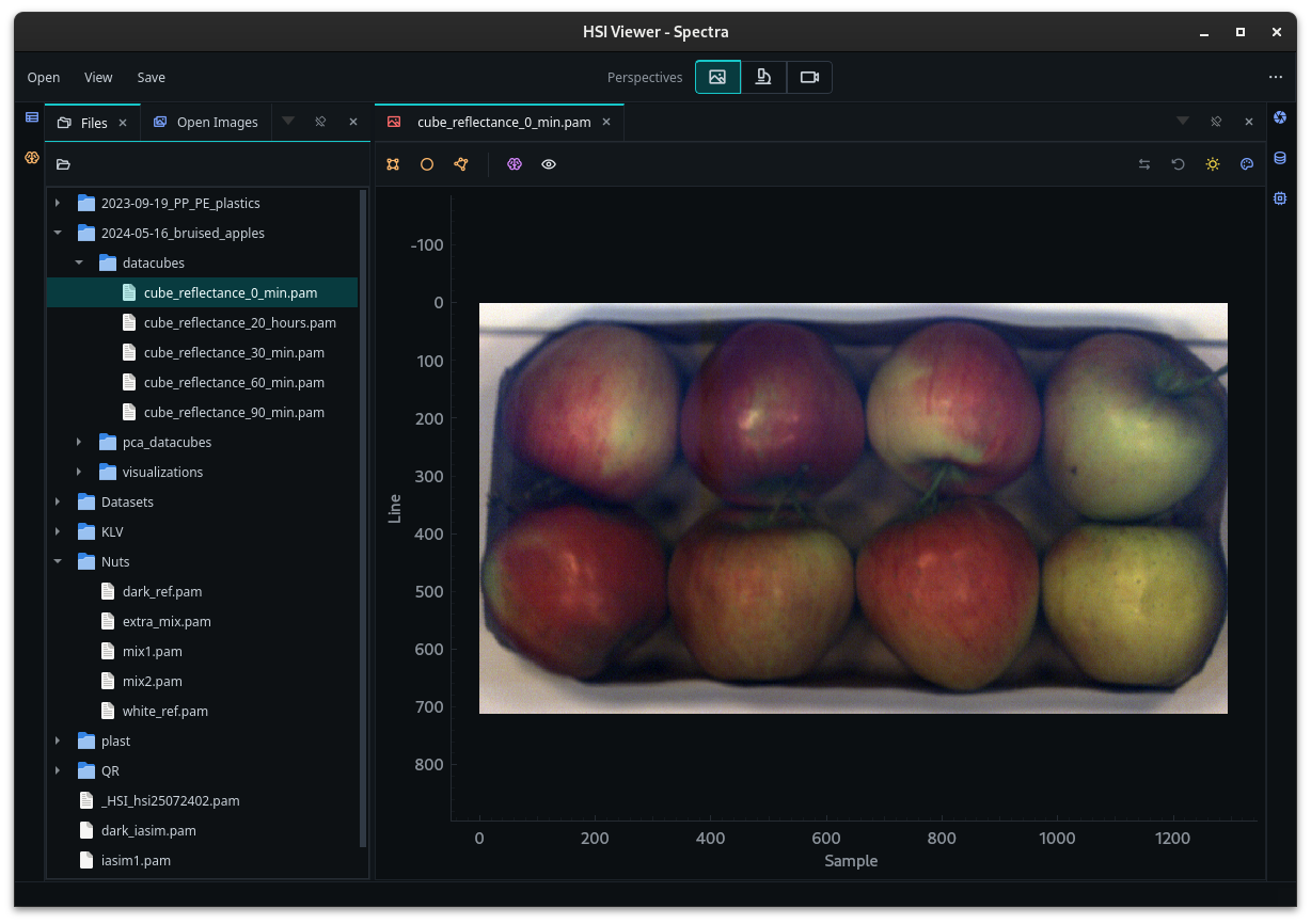
HV Explorer: bruised apples shown as false RGB

The bruised areas are difficult to identify in the false RGB preview. To inspect spectral variation across the complete image:

1. Add a PCA operation in the Workflow editor.
2. Select the number of components to calculate.
3. Apply the operation.
4. If the preview is in Color mode, change it to Gray mode.
5. Use the preview band/channel controls to inspect the resulting component images. Each band in the PCA result corresponds to one PCA component, so changing the selected band changes which component image is displayed.

In this example, component 5 makes the bruised regions clearly visible. Other components emphasize variations such as the separation between apples and the background. Component order and interpretation depend on the input data and any operations applied before PCA; component 5 will not generally represent bruising in other datasets.

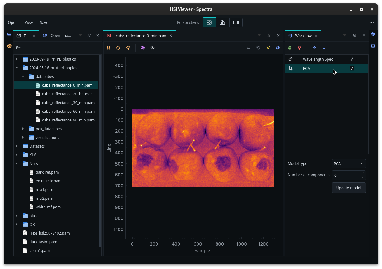
HV Explorer: bruised apples shown with PCA

See the PCA chapter for more information about scores, loadings, and component interpretation.

Demo

HV Explorer: PCA operation

Exporting datacubes

Use Save > Export current image to write the selected datacube and all currently enabled workflow operations to a new file. Export can therefore be used both to convert file formats and to save processed results such as calibrated, cropped, binned, band-selected, or model-generated cubes.

Export settings

1. Confirm in the Workflow editor which operations are enabled and in which order they will be applied.
2. Select Save > Export current image.
3. Choose the output format and interleave.
4. Select the destination and file name.
5. Start the export and wait for processing to complete.

Format	Common interleave	Notes
ENVI (.hdr)	BIL, BIP, or BSQ	Interleave is described by the ENVI header.
TIFF (.tif, .tiff)	BSQ	Naturally organized as a sequence of image planes.
PAM (.pam)	BIP	Stores each spatial pixel with its channel values.

HV Explorer and the HV SDK support BIL, BIP, and BSQ for all three formats. Other applications may assume the common layout shown above, so choose an interleave supported by the software that will consume the file. See Data ordering for a comparison of the layouts.

Check the output data type

Inspect the current data type in the Metadata inspector (#13) before export. Operations may change it; for example, reflectance calibration produces float32 values on an approximate [0, 1] scale.

If the target format or downstream application requires integer values, add a Scaling operation before export. This single operation applies the scale factor and converts the result to its selected target data type:

Target type	Scale for [0, 1] input	Trade-off
uint8	255	Smaller files with lower numerical precision.
uint16	65535	Higher precision with larger files.

PAM supports 8-bit and 16-bit integer output, so calibrated floating-point data must be scaled and converted before exporting to PAM. A separate DType Change operation is not required after Scaling. Use DType Change only for conversion without numerical rescaling.

See Scaling and type conversion for export for the reflectance-calibration example and recommended scale values. Avoid converting [0, 1] reflectance data directly to an integer type, because most values would be truncated to zero.

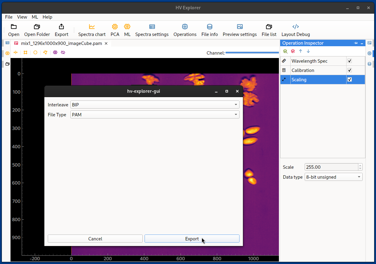
HV Explorer: exporting datacubes

Export is streamed

HV Explorer uses the HV SDK lazy processing model. The active workflow is computed and written progressively during export, so the complete processed cube does not need to be held in RAM at once.

Continue in Python

Exported datacubes can be opened with the HV SDK for scripted processing. See the basic examples for opening and visualization, or the preprocessing examples for band selection, binning, cropping, and saving processed cubes.