PCA and ML

This page introduces the analysis tools used after ROIs and properties have been created. Use PCA to check whether annotated groups separate spectrally, then train, preview, save, or apply machine-learning models from the same annotated data.

PCA view

The PCA view provides an exploratory comparison of spectra sampled from the current ROIs. Open it from View > PCA, or switch to the Analysis perspective if the pane is already included in that layout.

The PCA (Principal Component Analysis) is calculated from the pixels contained in the visible ROIs. Each point in the score plot represents a sampled pixel and is colored according to its ROI, or according to a selected annotation property. Clusters and overlap in the plot can therefore help reveal whether annotated groups have distinct spectral characteristics.

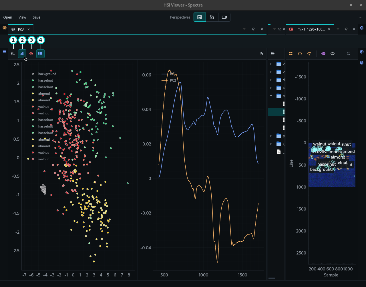
HV Explorer: PCA view

PCA controls

Number	Control	Description
1	Settings	Selects the number of components to calculate, the components shown on the X and Y axes, and whether points are grouped by annotations or a property.
2	Loadings	Shows or hides the loading curves for the selected components. Loadings indicate which wavelengths contribute most strongly to each component.
3	Point highlight	Shows or hides the point under the mouse cursor as a blue cross in the score plot.
4	Legend	Shows or hides the plot legend.

The PCA result is recalculated automatically when ROIs are changed, removed, hidden, or shown. Changing the selected property or PCA components also updates the visualization.

Interpreting the result

Points that form separate clusters indicate spectral differences between the sampled groups. Strong overlap suggests that the selected spectra are not well separated by the displayed components. Check other component combinations and inspect the loading curves to identify wavelengths responsible for the observed variation.

In this example, the background forms a distinct cluster, while the walnut samples overlap considerably with both the almonds and hazelnuts samples. Changing the displayed components does not produce clear separation. Applying preprocessing such as SNV in the Workflow editor may reduce intensity and scattering variation and improve the grouping. The PCA view is recalculated using the processed data after the workflow changes.

Use representative ROIs

PCA reflects only the pixels included in the visible ROIs. Use representative ROIs and avoid including unwanted background pixels, shadows, or mixed sample regions when comparing groups.

PCA view and PCA operation

The PCA view is an interactive analysis tool based on ROI samples. The PCA operation instead applies PCA to the datacube and returns component images that can be used in the processing workflow or exported.

Demo

HV Explorer: PCA view

ML Trainer

The ML Trainer creates classification, regression, and clustering models from spectra sampled from annotations. Open it from View > ML trainer, or switch to the Analysis perspective if the pane is already included in that layout.

Prepare training data

Create representative ROIs for the samples used to train the model. Training can use ROIs from the current datacube or from multiple open datacubes.

For supervised models, add an annotation property that contains the desired target value:

• Use a label property for classification, with values such as almond, walnut, and hazelnut.
• Use a numeric property for regression, with values such as moisture or concentration.

Assign the appropriate property value to every ROI used for training. If each class is represented by exactly one ROI, classification can also use the ROI annotations directly by selecting None as the target property.

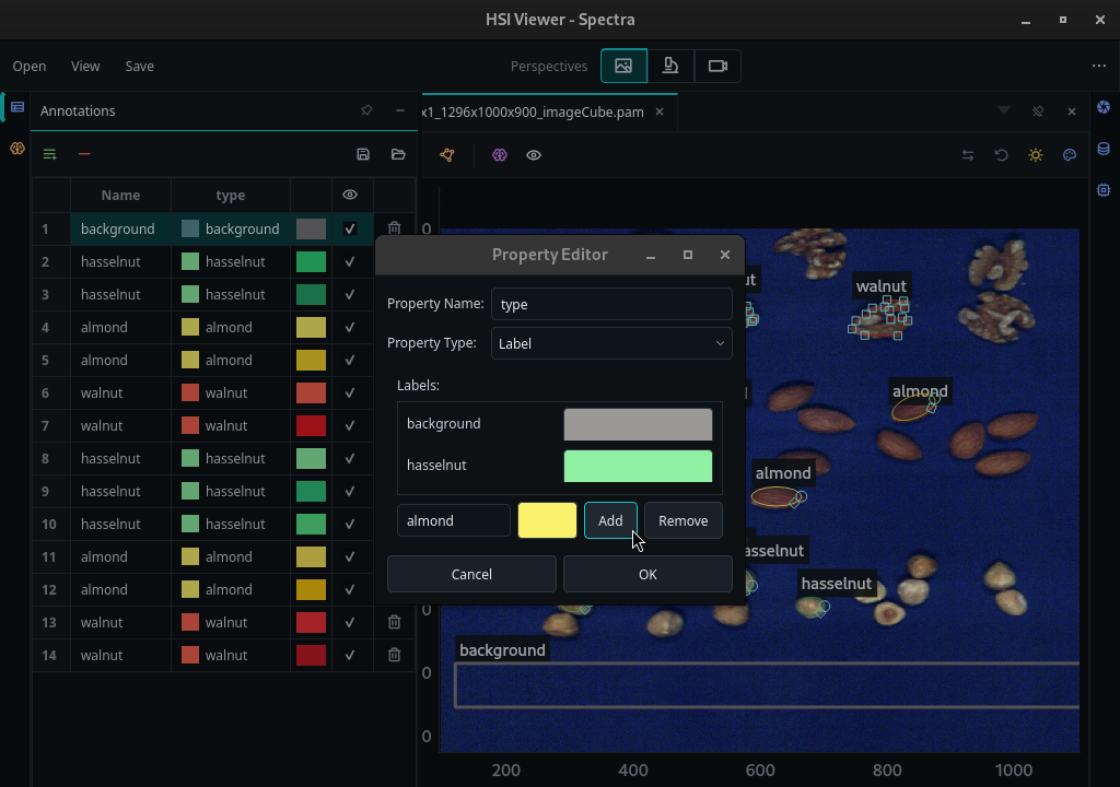
HV Explorer: Add property

Keep training and application data consistent

Models learn from spectra after the currently enabled workflow operations have been applied. Use the same reflectance calibration, preprocessing, band selection, binning, and wavelength order when evaluating or applying the model to another datacube. Spatial crop or binning operations can also change ROI coordinates and may require annotations to be adjusted.

Create and train a model

1. Click the green Add model button in the ML Trainer toolbar.
2. Select the Target property used for classification or regression.
3. Set the Sample size and select a Model type.
4. Configure the parameters shown for the selected model.
5. Click Train and wait for the progress indicator to reach 100%.

To rename a model, double-click its name in the Models list and enter the new name.

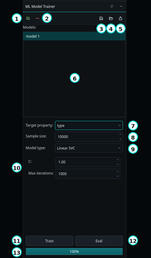
HV Explorer: ML Trainer

ML Trainer controls

Number	Control	Description
1	Add model	Add a new model to the model list.
2	Remove model	Remove the selected model from the model list.
3	Save model	Save the selected model as an HV Explorer model file.
4	Load model	Load a previously saved HV Explorer model.
5	Export model	Export the selected trained model for use outside HV Explorer.
6	Model list	Show the available models. Select a model to configure it, or double-click its name to rename it.
7	Target property	Select the annotation property used as the classification or regression target.
8	Sample size	Set the number of ROI spectra sampled for training.
9	Model type	Select the machine-learning algorithm.
10	Model settings	Configure parameters specific to the selected model type.
11	Train	Train the selected model using the current annotations and settings.
12	Eval	Run the experimental model-evaluation action.
13	Progress bar	Show the training progress and completion percentage.

Model types

Task	Available models	Target
Classification	Linear SVC, PLS-DA	Label property or ROI annotations
Regression	SVR, Least squares, Regularized least squares	Numeric property
Clustering	KMeans	No supervised target required

The appropriate model depends on the target, available training data, and the spectral relationship being modeled.

Experimental evaluation

The Eval button is currently experimental and does not provide a supported evaluation report in the interface. PLS-DA evaluation is not implemented. Until this is expanded, validate trained models on independent annotated datacubes and inspect their predictions critically before deployment.

Managing models

The ML Trainer toolbar provides three ways to preserve or reuse a model:

Action	Purpose
Save model	Saves an HV Explorer model file containing the trained estimator and the target-property information.
Load model	Restores a model previously saved by HV Explorer.
Export model	Exports the underlying trained scikit-learn estimator for use in Python.

The supported Python export is currently SciKit-Learn (.pkl). Although ONNX appears in the export dialog, ONNX export is not currently implemented and should not be used.

Saving or exporting a model does not include the datacube processing pipeline. Record and reproduce the calibration, preprocessing, band selection, binning, and wavelength order separately.

Preview model results

Click the purple Model overlay icon in the image toolbar and select a trained model. HV Explorer evaluates the current datacube and displays the result as an overlay. For classification, the overlay uses the colors assigned to the target labels.

Use the adjacent eye icon to show or hide the selected overlay. This makes it possible to compare predictions with the preview and annotations without retraining the model.

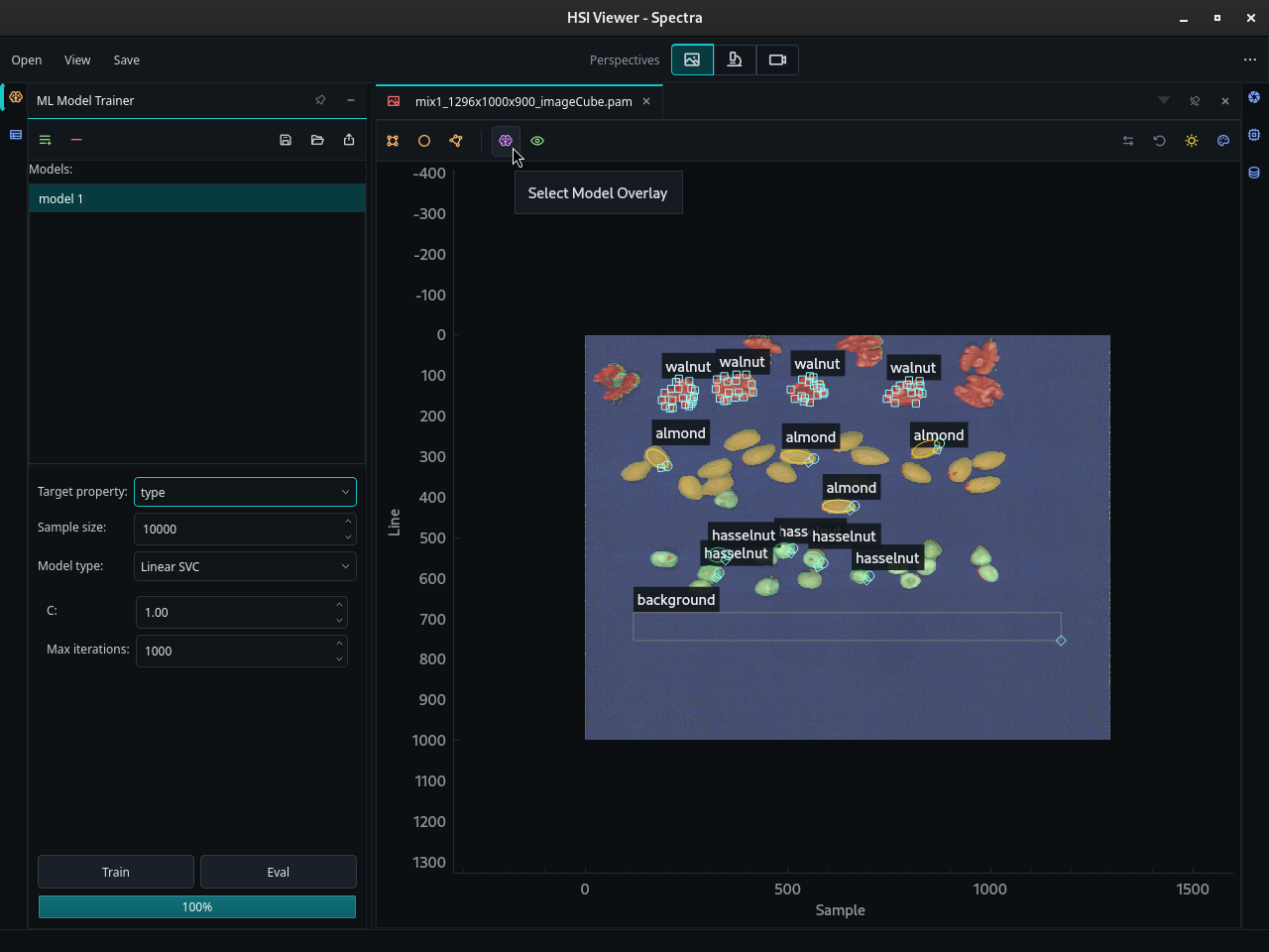
HV Explorer: ML Preview

Apply a model as an operation

To create a processed result instead of a temporary preview overlay:

1. Disable the model overlay.
2. Add ML > Apply ML model in the Workflow editor.
3. Select the trained model in the operation settings.
4. Click Apply model.
5. Switch the preview to Gray mode to display the operation result. If the preview remains in Color mode, it continues to show the selected false RGB channels instead.

For classification models, the operation generates a classification result that can be inspected in the Gray preview.

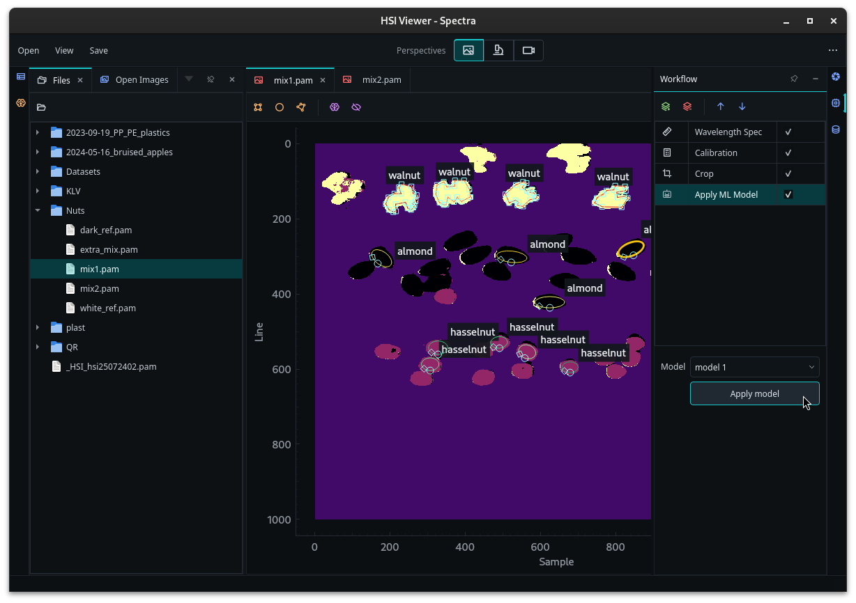
HV Explorer: Apply ML model

The overlay and operation can also be applied to other open datacubes, allowing a model trained from one or more cubes to be tested on separate data.

Using exported models in Python

See Load a model exported from HV Explorer for a complete HV SDK example using a SciKit-Learn export. Reproduce the same processing pipeline before applying the estimator.

Demo

HV Explorer: ML Trainer