Annotations and Spectra
This page shows how to mark regions of interest, assign labels or numeric properties, and compare spectra from selected sample areas. These annotations become the link between visual inspection, spectral analysis, PCA, ML training, and later SDK workflows.
Annotations
Annotations define regions of interest (ROIs) within a datacube. Each annotation selects spatial pixels that can be reused throughout the analysis workflow. For example, annotations can be used to:
- Calculate and compare mean spectra in the Spectral Viewer.
- Sample pixels for the PCA view and inspect grouping, separation, and loadings.
- Provide training data for classification or regression models.
- Save reusable ROI definitions for later HV Explorer sessions or HV SDK workflows.
Creating ROIs
The preview toolbar provides three ROI tools. Select a tool, then place and adjust the ROI over the sample region you want to analyze.
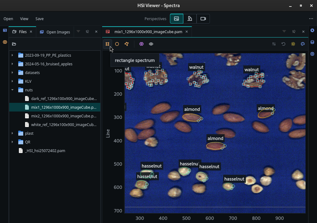
HV Explorer: creating ROIs
| ROI tool | Description |
|---|---|
| Rectangular ROI | Creates a rectangular region. Move or resize it to cover the desired sample area. |
| Elliptical ROI | Creates an elliptical region. Its position, size, and angle can be adjusted. |
| Polygonal ROI | Creates a free-form region from multiple points. Press Enter or click the first point to close the polygon. |
After creating a polygon, drag its points to adjust the shape. Click a line segment to add a point. To remove a point, right-click it and select Remove handle.
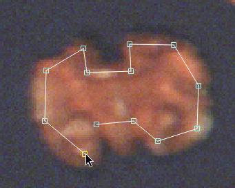
Polygonal ROI editing
Annotation settings
Open the Annotations panel (#6) to manage the ROIs in the current session. Each annotation has a name and color, and can be selected, shown/hidden, assigned properties, saved/loaded, or deleted. Selecting an annotation also highlights its ROI in the preview and its corresponding curve in the Spectral Viewer.
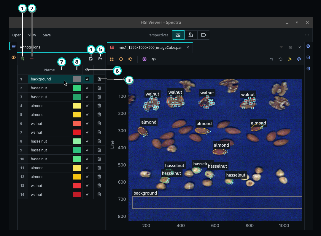
HV Explorer: Annotations panel
Double-click an annotation name to rename it, or double-click its color to open the color picker. Descriptive names and consistent colors make annotations easier to recognize in spectral plots, PCA views, and ML workflows.
| Number | Control | Description |
|---|---|---|
| 1 | Add property | Create a label or numeric property. Properties appear as additional annotation columns and can be used to group or target data for PCA and ML. |
| 2 | Remove property | Remove the selected property from the annotation table. |
| 3 | Delete annotation | Delete the selected annotation or annotations. The Del key can also remove all selected annotations at once. |
| 4 | Save annotations | Save ROI geometry, names, colors, and properties to a JSON file. |
| 5 | Load annotations | Load annotations from JSON and append them to the current annotation list. |
| 6 | Show/hide annotation | Toggle whether the selected annotation is included in the Spectral Viewer. |
| 7 | Annotation name | Identifies the annotation; double-click to edit. |
| 8 | Annotation color | Controls the ROI and plot color; double-click to change it. |
Hiding an annotation keeps its ROI and metadata but removes it from the spectral
plot. Deleting an annotation removes it from the current session. Select one or
more annotations and press the Del key to remove all selected ROIs at once.
The delete button (#3) performs the same action.
Use hiding when you may want to restore an annotation later; use deletion when the ROI is no longer needed.
Annotation properties
Properties add categorical or numeric information to each annotation. They can later be selected in PCA, classification, and regression workflows.
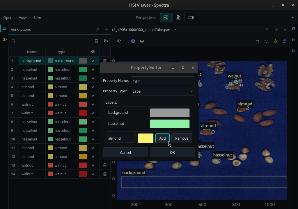
HV Explorer: Annotations panel
To create and assign a property:
- Click Add property (#1) in the Annotations panel.
- Enter the desired property name.
- Select the property type:
- Label creates a categorical property with a predefined set of choices,
such as
almond,walnut, orhazelnut. Use labels to group ROIs into classes for PCA or classification. - Value creates a numeric property for continuous measurements or target values, such as moisture or concentration. Use values for regression or other analyses based on numeric metadata.
- Label creates a categorical property with a predefined set of choices,
such as
- For a Label property, type a label name, select its color, and click Add. Repeat this for each label that should be available.
- Click OK when the property is configured.
The property appears as a new column in the annotation table. Double-click the property cell for an ROI, then select the appropriate choice for a Label property or enter the numeric target for a Value property. Repeat this for each ROI that should have the property assigned.
Right-click a value in a property column and select Edit property to change the available labels. Editing a property resets its assignments, so the values must then be reassigned to the relevant ROIs.
Saving and loading annotations
Click Save annotations (#4) to save the current ROI geometry, names, colors, and properties to a JSON file. Use this file to continue the analysis in a later session, apply the same ROIs to another datacube, or reuse the annotations with the HV SDK.
Click Load annotations (#5) and select a saved annotation JSON file to load it. The loaded annotations are appended to the current annotation list rather than replacing existing annotations.
Annotation JSON files can also be used with the HV SDK annotation examples, classification examples, regression examples, and PCA examples.
Demo
HV Explorer: Creating ROIs and mangaging annotations
Spectral Viewer
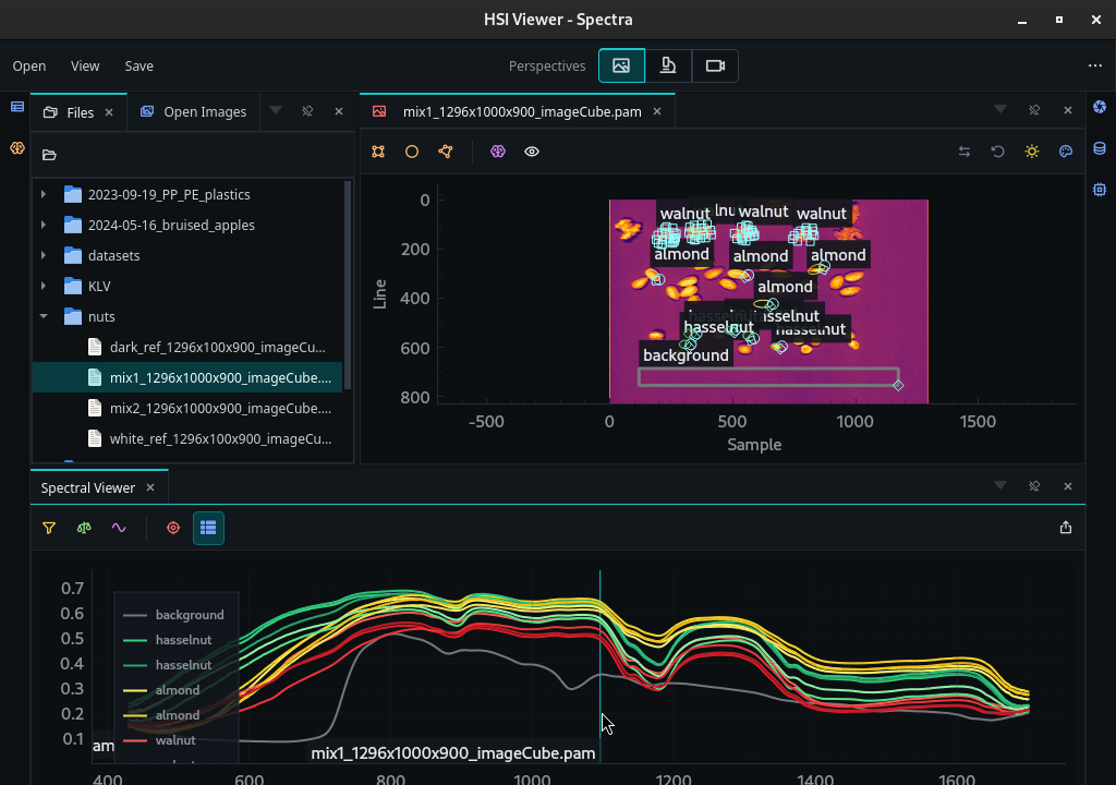
After creating one or more ROIs, open Spectral Viewer from the View Menu (#2). The viewer plots the mean spectrum of each visible annotation, using the annotation name and color from the Annotations panel.
HV Explorer: Spectral Viewer
Selecting an annotation in the Annotations panel highlights both its ROI in the preview and its curve in the plot. Selecting a curve or its legend entry in the Spectral Viewer highlights the corresponding annotation. This makes it easy to move between spatial regions and their spectral signatures.
Use the visibility controls in the Annotations panel to show or hide individual ROI spectra. The legend can be shown or hidden from the Spectral Viewer toolbar.
Enable the crosshair control to plot the spectrum of the pixel under the mouse cursor. This is useful for inspecting individual pixels before creating an ROI.
When the preview is in grayscale mode, the cyan vertical line in the spectral plot indicates the band or wavelength currently displayed in the preview. Drag the line horizontally across the plot to select a different band and update the grayscale preview.
When wavelength metadata is available, the horizontal axis displays wavelength in nanometers. Otherwise, the plot uses the band/channel index. Add wavelength metadata with the Setup Wizard or the Wavelength Spec operation.
Spectra settings
The Spectral Viewer toolbar provides controls for smoothing, preprocessing, uncertainty display, point inspection, legend visibility, and data export. These settings affect the plotted spectra only; they do not modify the datacube or its processing pipeline in the Workflow editor.
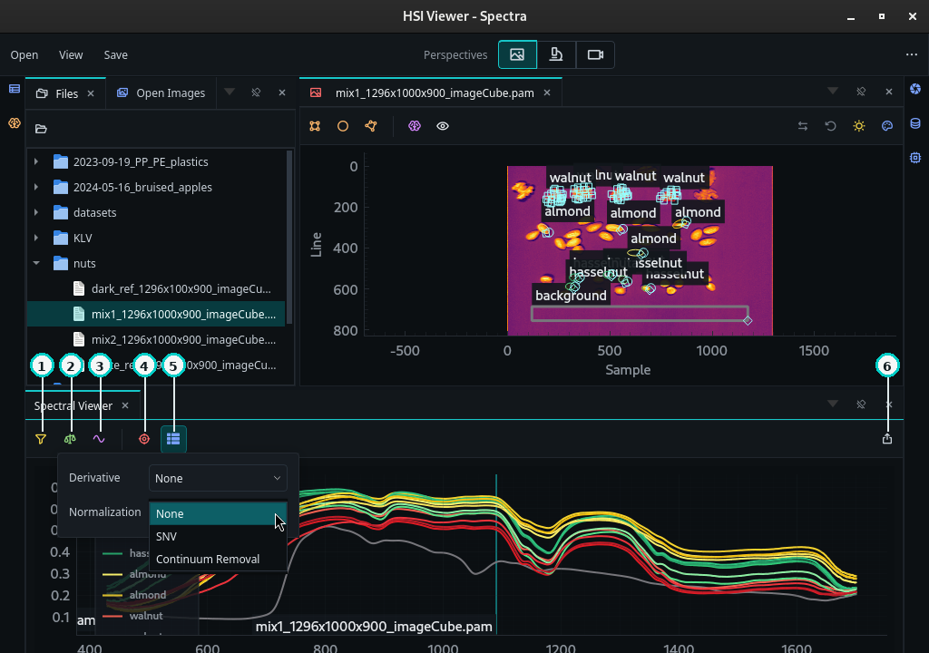
HV Explorer: Spectra settings interface
| Number | Control | Description |
|---|---|---|
| 1 | Smoothing filter | Smooth the plotted spectra using a Gaussian or Savitzky-Golay filter. |
| 2 | Spectral preprocessing | Apply SNV, continuum removal, or a first- or second-order derivative to the plotted spectra. |
| 3 | Standard deviation | Show or hide the standard deviation calculated from the pixels within each ROI. |
| 4 | Point spectrum | Show or hide the spectrum of the pixel beneath the mouse cursor in the preview image. |
| 5 | Legend | Show or hide the plot legend. |
| 6 | Export | Open a menu to export spectra as CSV, XLSX, or JSON in wide or long layout, or export the current plot as a Matplotlib plot. |
Spectral Viewer filters and preprocessing affect only the displayed and exported spectra. They do not change PCA, ML, preview, or datacube export input. To apply preprocessing to every pixel, use an available operation in the Workflow editor, such as SNV.
Spectra and ROI exports can be reused directly in the HV SDK examples:
| Export from HV Explorer | File type | Typical SDK use |
|---|---|---|
| Save annotations | JSON | Load ROIs with the annotation examples or use them for classification, regression, and PCA. |
| Export spectra data | CSV, XLSX, JSON | Train from exported mean spectra in the classification example. |
Comparing spectra
Create ROIs for the almonds, walnuts, and hazelnuts and compare their mean spectra. Start with the calibrated spectra, then use the Spectral Viewer preprocessing controls to explore whether normalization or derivatives make subtle differences easier to identify.
With SNV enabled, the overall spectral shapes remain similar, but differences can be seen around 1150 nm and 1400 nm.
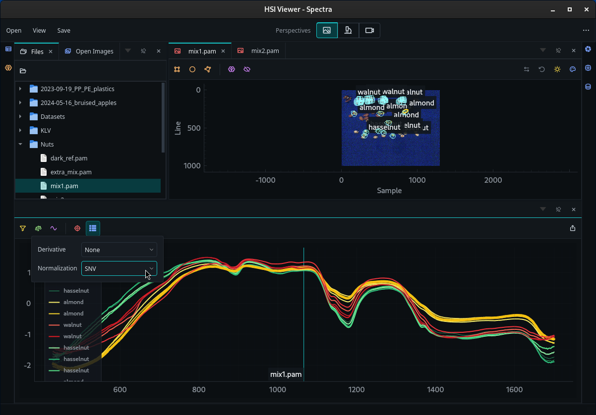
HV Explorer: spectra of almonds, walnuts and hazelnuts
Right-click the plot area and select Plot options -> Grid to show or hide the horizontal and vertical grid lines.
Applying the first derivative can make subtle differences easier to see. In this example, stronger separation appears around 1150 nm, 1200 nm, and 1350 nm.
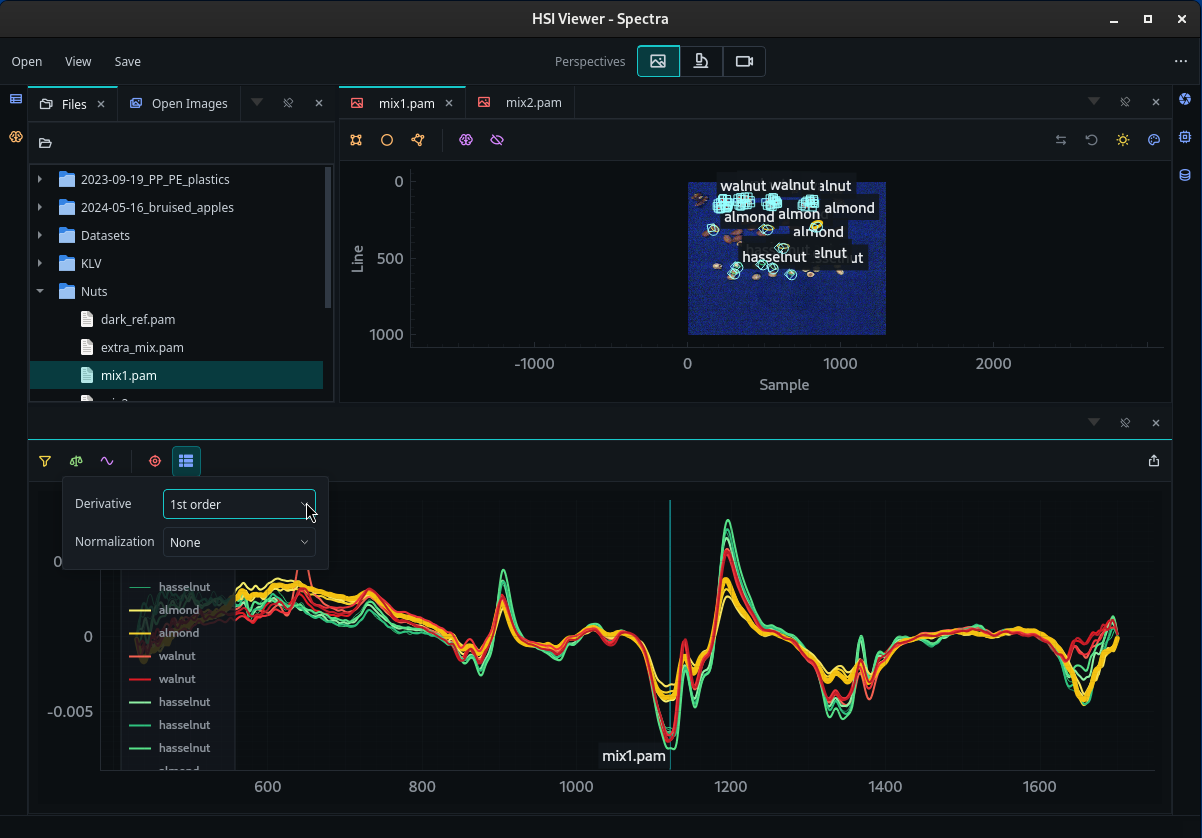
HV Explorer: spectra of almonds versus walnuts (1st derivative)
Demo
HV Explorer: Spectral Viewer